CMPT 706 Algorithms for Big Data Dynamic Programming

CMPT 706 - Algorithms for Big Data Dynamic Programming March 24, 2020 Dynamic Programming 1 -1

Dynamic Programming A general paradigm that in which a problem is solved by • breaking it into smaller subproblems • tackling them one by one, smallest first • using the answers to small subproblems solve the larger problem Similar to the divide-and-conquer paradigm using recursion However, instead of recursive calls we use memorization. Dynamic Programming 1 -2

A simple example Fibonacci sequence Approximation Algorithms 1 -3

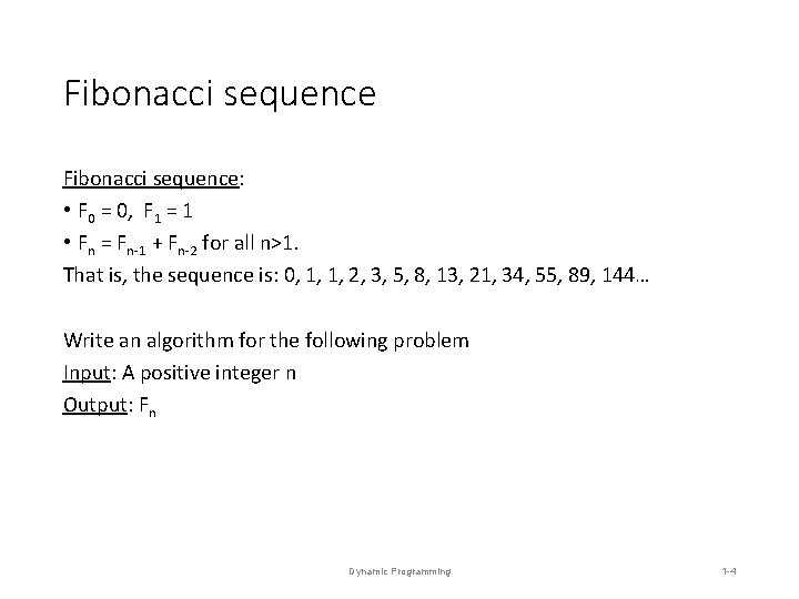
Fibonacci sequence: • F 0 = 0, F 1 = 1 • Fn = Fn-1 + Fn-2 for all n>1. That is, the sequence is: 0, 1, 1, 2, 3, 5, 8, 13, 21, 34, 55, 89, 144… Write an algorithm for the following problem Input: A positive integer n Output: Fn Dynamic Programming 1 -4

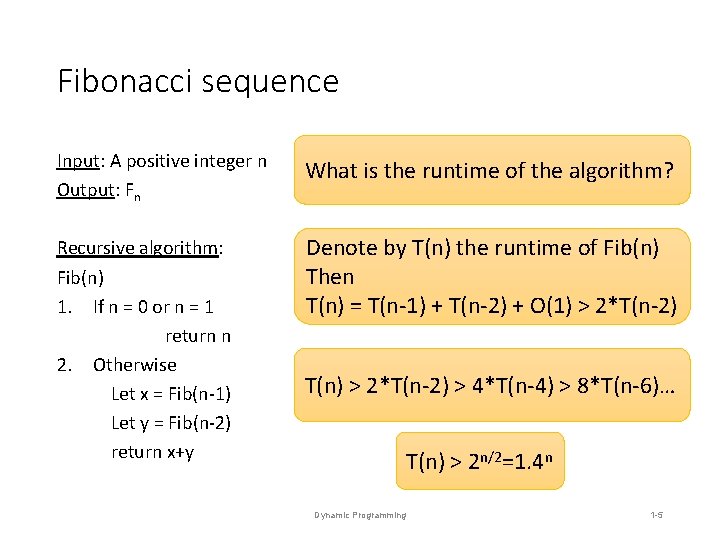
Fibonacci sequence Input: A positive integer n Output: Fn What is the runtime of the algorithm? Recursive algorithm: Fib(n) 1. If n = 0 or n = 1 return n 2. Otherwise Let x = Fib(n-1) Let y = Fib(n-2) return x+y Denote by T(n) the runtime of Fib(n) Then T(n) = T(n-1) + T(n-2) + O(1) > 2*T(n-2) T(n) > 2*T(n-2) > 4*T(n-4) > 8*T(n-6)… T(n) > 2 n/2=1. 4 n Dynamic Programming 1 -5

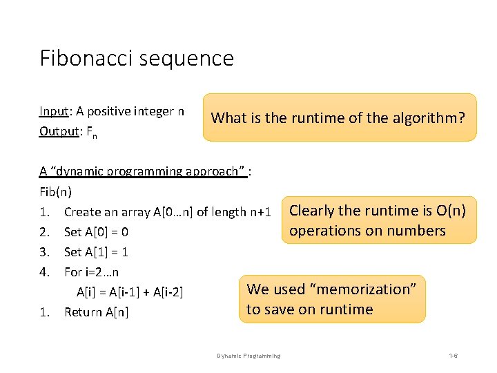
Fibonacci sequence Input: A positive integer n Output: Fn What is the runtime of the algorithm? A “dynamic programming approach” : Fib(n) 1. Create an array A[0…n] of length n+1 Clearly the runtime is O(n) operations on numbers 2. Set A[0] = 0 3. Set A[1] = 1 4. For i=2…n We used “memorization” A[i] = A[i-1] + A[i-2] to save on runtime 1. Return A[n] Dynamic Programming 1 -6

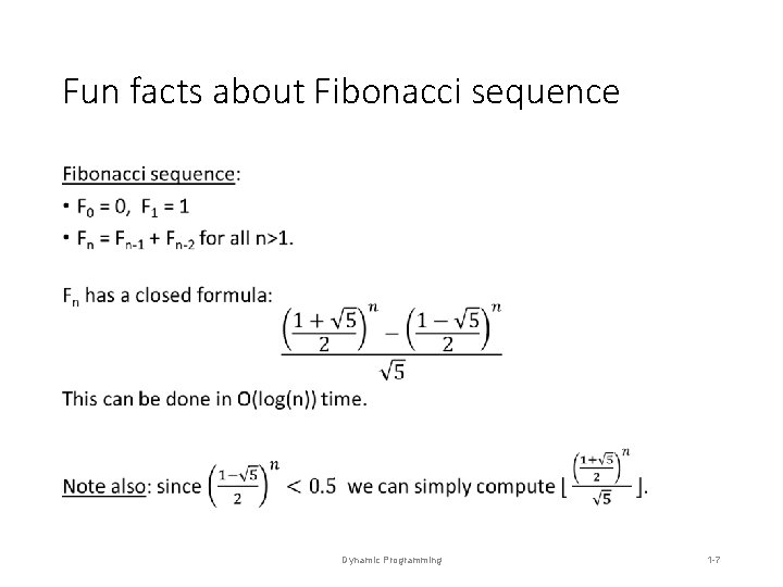
Fun facts about Fibonacci sequence • Dynamic Programming 1 -7

The shortest path problem (again) Approximation Algorithms 1 -8

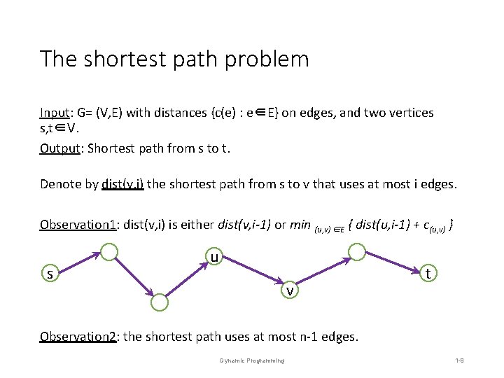
The shortest path problem Input: G= (V, E) with distances {c(e) : e∈E} on edges, and two vertices s, t∈V. Output: Shortest path from s to t. Denote by dist(v, i) the shortest path from s to v that uses at most i edges. Observation 1: dist(v, i) is either dist(v, i-1) or min (u, v)∈E { dist(u, i-1) + c(u, v) } s u v t Observation 2: the shortest path uses at most n-1 edges. Dynamic Programming 1 -9

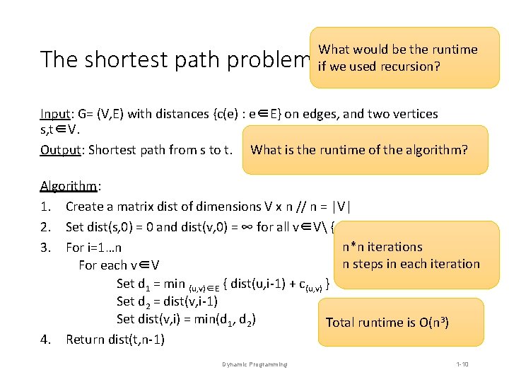
The shortest path problem What would be the runtime if we used recursion? Input: G= (V, E) with distances {c(e) : e∈E} on edges, and two vertices s, t∈V. Output: Shortest path from s to t. What is the runtime of the algorithm? Algorithm: 1. Create a matrix dist of dimensions V x n // n = |V| 2. Set dist(s, 0) = 0 and dist(v, 0) = ∞ for all v∈V {s} n*n iterations 3. For i=1…n n steps in each iteration For each v∈V Set d 1 = min (u, v)∈E { dist(u, i-1) + c(u, v) } Set d 2 = dist(v, i-1) Set dist(v, i) = min(d 1, d 2) Total runtime is O(n 3) 4. Return dist(t, n-1) Dynamic Programming 1 -10

The Knapsack problem Approximation Algorithms 1 -11

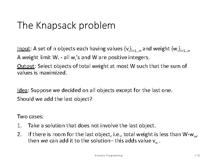
The Knapsack problem Input: A set of n objects each having values {vi}i=1…n and weight {wi}i=1…n A weight limit W. - all wi’s and W are positive integers. Output: Select objects of total weight at most W such that the sum of values is maximized. Idea: Suppose we decided on all objects except for the last one. Should we add the last object? Two cases: 1. Take a solution that does not involve the last object. 2. If there is room for the last object, i. e. , total weight is less than W-w n, then we can add it to the solution– this adds value vn. Dynamic Programming 1 -12

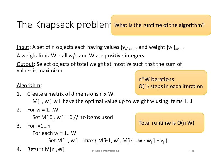
The Knapsack problem What is the runtime of the algorithm? Input: A set of n objects each having values {vi}i=1…n and weight {wi}i=1…n A weight limit W - all wi’s and W are positive integers Output: Select objects of total weight at most W such that the sum of values is maximized. n*W iterations Algorithm: O(1) steps in each iteration 1. Create a matrix of dimensions n x W M[ i, w ] will have the optimal value up to weight w using items 1…i 2. For w = 1…W Set M[ 0 , w ] = 0 // no items used Total runtime is O(n W) 3. For i=1…n For each w = 1…W Set M[ i , w ] = max ( M[i-1, w], M[i-1, w - wi ] + vi ) 4. Return M[n , W] Dynamic Programming 1 -13

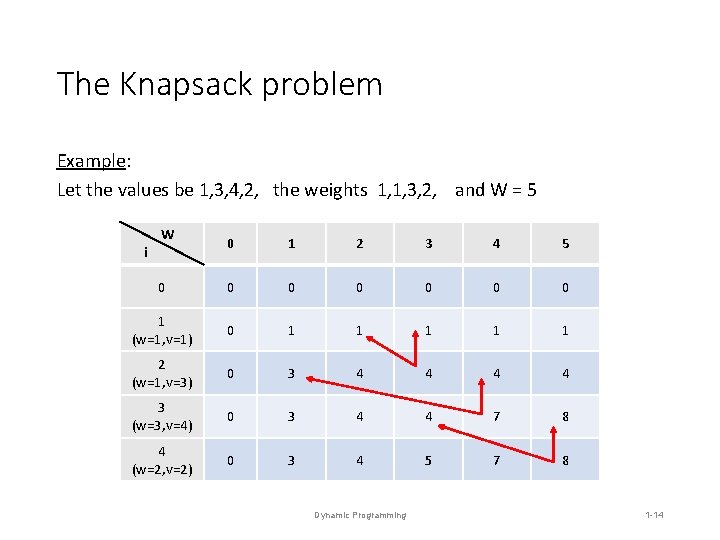
The Knapsack problem Example: Let the values be 1, 3, 4, 2, the weights 1, 1, 3, 2, and W = 5 W 0 1 2 3 4 5 0 0 0 0 1 (w=1, v=1) 0 1 1 1 2 (w=1, v=3) 0 3 4 4 3 (w=3, v=4) 0 3 4 4 7 8 4 (w=2, v=2) 0 3 4 5 7 8 i Dynamic Programming 1 -14

Reading for next time Exercises from the Book: 6. 2, 6. 3, 6. 6 Reading 6. 2, 6. 3 Huffman Code 1 -15