CMPT 225 Lecture 11 Quick Sort Last Lecture

CMPT 225 Lecture 11 – Quick Sort

Last Lecture We saw how … Merge sort works To define the best, worst, and average case running time and space efficiency of merge sort 2

Learning Outcomes At the end of the next few lectures, a student will be able to: describe the behaviour of and implement simple sorting algorithms: insertion sort selection sort describe the behaviour of and implement more efficient sorting algorithms: quick sort merge sort analyze the best, worst, and average case running time (and space) of these sorting algorithms 3

Today’s menu Looking at Describing how quick sort function Analyzing the time efficiency of quick sort Discussing how to improve quick sort’s time efficiency Analyzing its space efficiency Discussing how to improve quick sort’s space efficiency 4

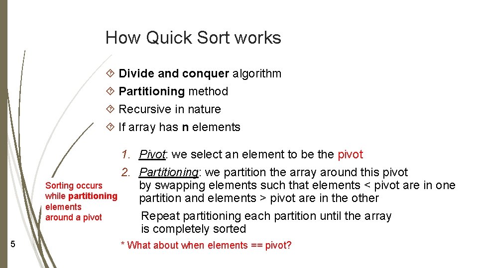
How Quick Sort works Divide and conquer algorithm Partitioning method Recursive in nature If array has n elements 1. Pivot: we select an element to be the pivot 2. Partitioning: we partition the array around this pivot Sorting occurs by swapping elements such that elements < pivot are in one while partitioning partition and elements > pivot are in the other elements Repeat partitioning each partition until the array around a pivot is completely sorted 5 * What about when elements == pivot?

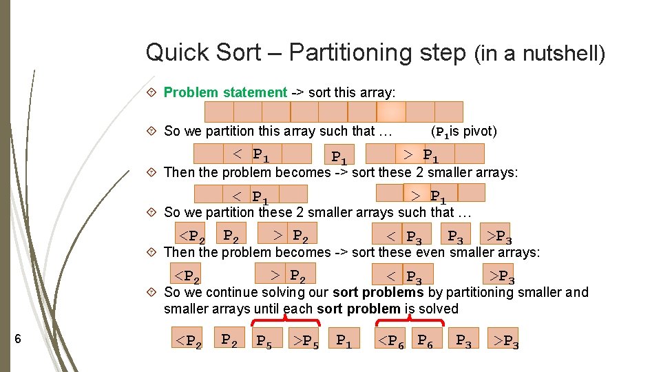
Quick Sort – Partitioning step (in a nutshell) Problem statement -> sort this array: So we partition this array such that … < P 1 (P 1 is pivot) > P 1 Then the problem becomes -> sort these 2 smaller arrays: > P 1 < P 1 So we partition these 2 smaller arrays such that … <P 2 > P 2 < P 3 P 3 >P 3 Then the problem becomes -> sort these even smaller arrays: <P 2 >P 3 So we continue solving our sort problems by partitioning smaller and smaller arrays until each sort problem is solved 6 <P 2 P 5 >P 5 P 1 <P 6 P 3 >P 3

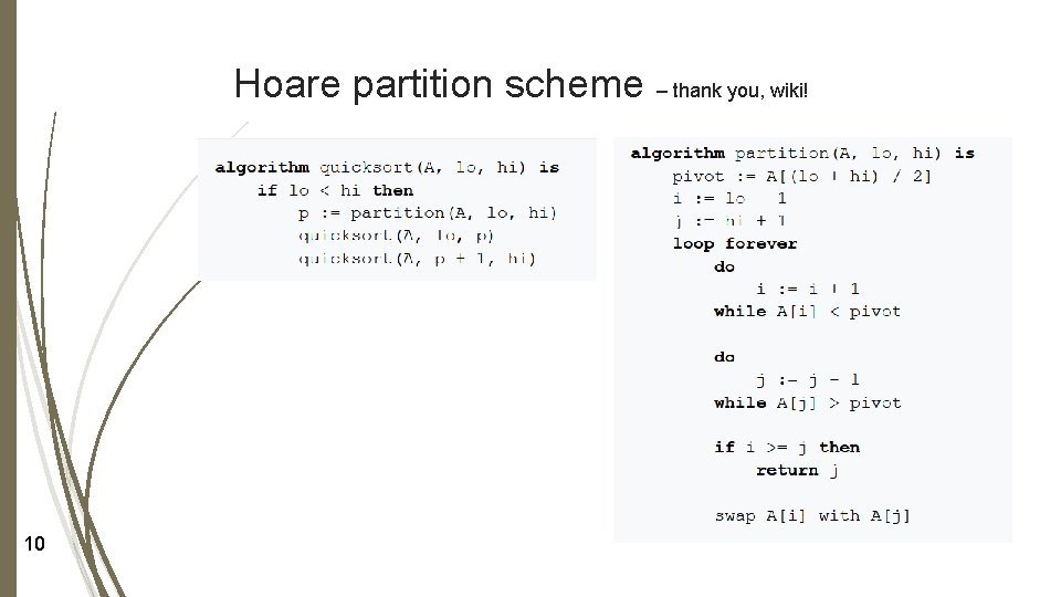
Many different versions of Quick Sort Different ways of selecting the pivot Will be discuss later on in lecture notes Different ways of partitioning the array using the pivot Lomuto partition scheme Hoare partition scheme 7

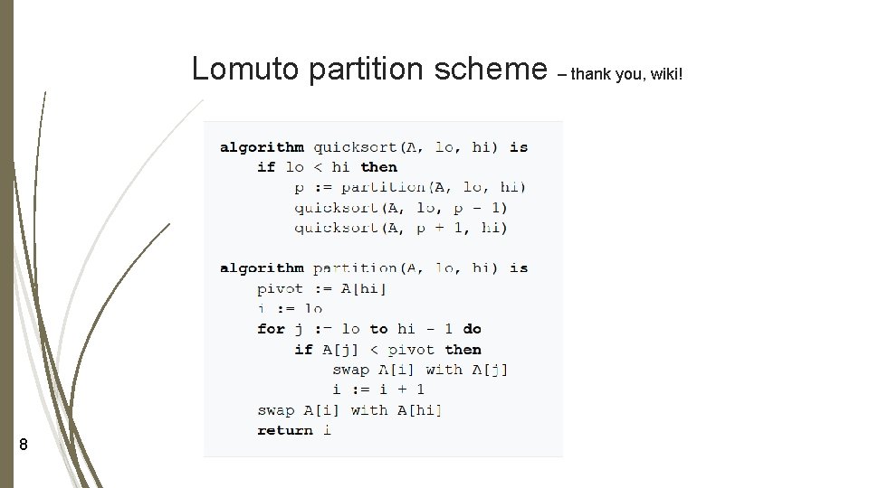
Lomuto partition scheme – thank you, wiki! 8

Demo - Let’s have a look at Quick Sort Lomuto partition scheme 9

Hoare partition scheme – thank you, wiki! 10

Demo - Let’s have a look at Quick Sort Hoare partition scheme 11

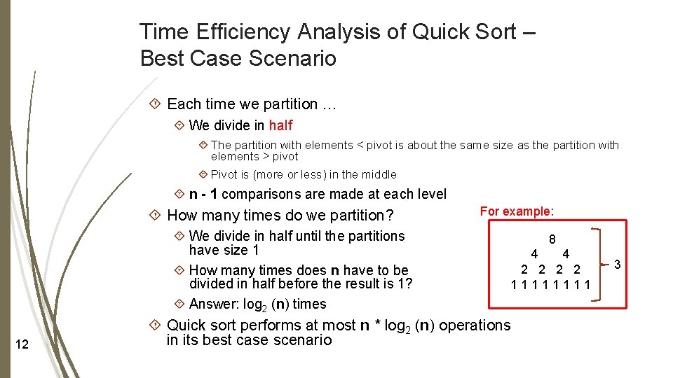
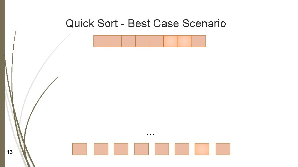
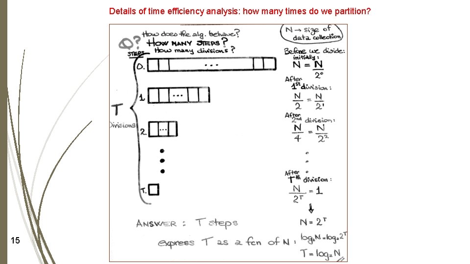
Time Efficiency Analysis of Quick Sort – Best Case Scenario Each time we partition … We divide in half The partition with elements < pivot is about the same size as the partition with elements > pivot Pivot is (more or less) in the middle n - 1 comparisons are made at each level How many times do we partition? We divide in half until the partitions have size 1 How many times does n have to be divided in half before the result is 1? Answer: log 2 (n) times 12 For example: 8 4 4 2 2 1111 Quick sort performs at most n * log 2 (n) operations in its best case scenario 3

Quick Sort - Best Case Scenario … 13

Why at most? 14

Details of time efficiency analysis: how many times do we partition? 15

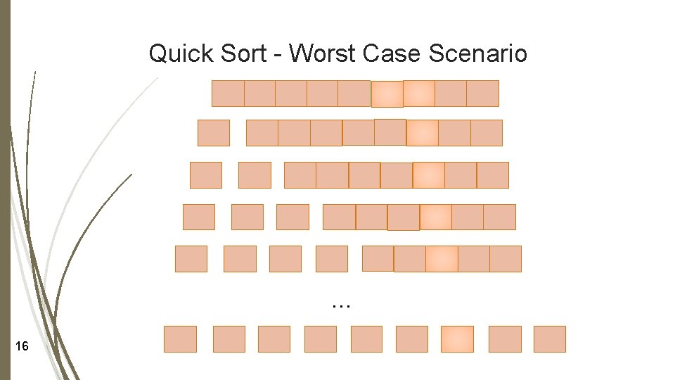
Quick Sort - Worst Case Scenario … 16

Time Efficiency Analysis of Quick Sort – Worst Case Scenario Each time we partition … We don’t divide in half Either the partition with elements < pivot is empty or the partition with elements > pivot is empty Pivot, when swapped, lands at either end of the partition n - 1 comparisons are made at each level How many times do we partition? Every time we partition, all we do is remove the pivot from the partition So every time we partition, we decrement the size of the partition (n) by 1 How many times does n have to be decremented by 1 before it reaches 1? Answer: n - 1 times (or n - 1 partition) 17 Quick sort performs n - 1 * n - 1 operations -> n 2 operations in its worst case scenario For example: If n = 8: 8 7 6 5 4 3 2 1 7

Time Efficiency Analysis of Quick Sort – Average Case Scenario Average case scenario of quick sort is closer to its best case scenario than to its worst case scenario 18

Time Efficiency Analysis of Quick Sort Time efficiency of Best case: Average case: Worst case: Does the organization of the data in the array to be sorted affect the amount of work done by quick sort? 19

Improving Quick Sort – Choice of Pivot Different ways of selecting the pivot: Way 1 (used so far): array[0] or array[size-1] Way 2: use largest of 1 st two elements Advantage of ways 1 and 2: Disadvantage of ways 1 and 2: 20

Improving Quick Sort – Choice of Pivot Way 3: choose three elements First, last and middle elements of array Sort order them Pick their median as pivot O(1) Advantage: Disadvantage: 21 To be used if problem statement leads us to believe that the array may be partially sorted

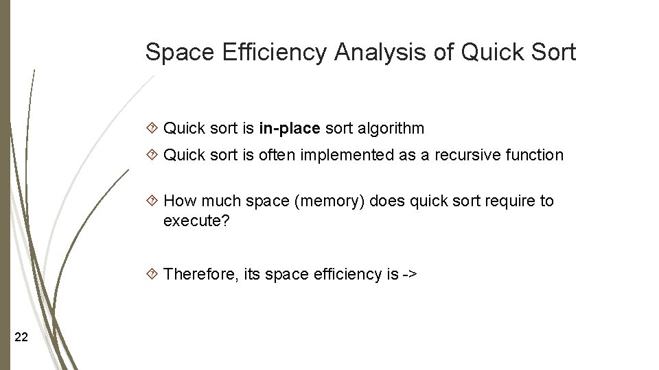
Space Efficiency Analysis of Quick Sort Quick sort is in-place sort algorithm Quick sort is often implemented as a recursive function How much space (memory) does quick sort require to execute? Therefore, its space efficiency is -> 22

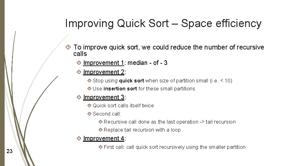
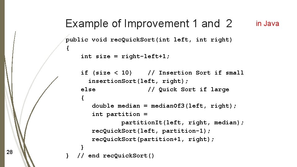
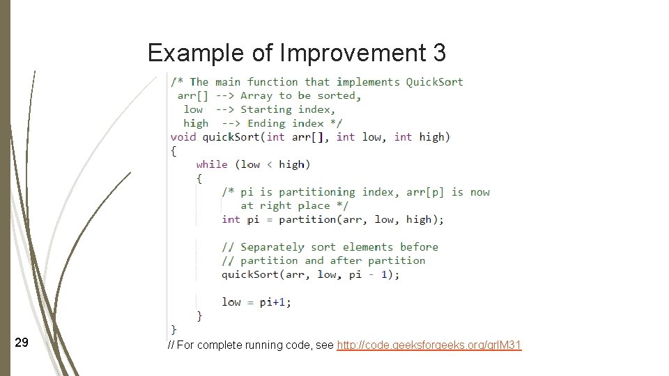
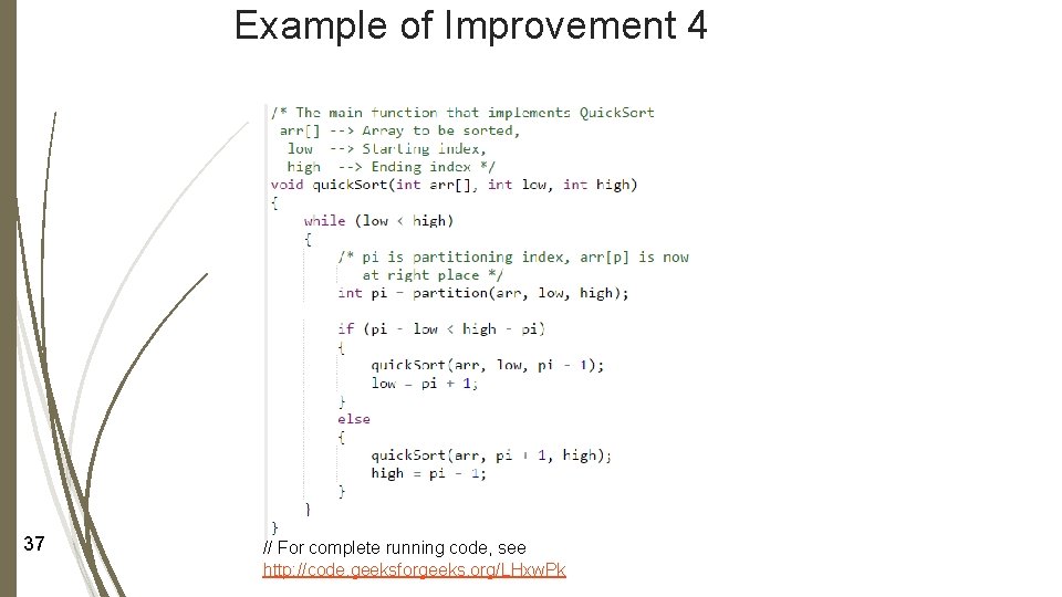
Improving Quick Sort – Space efficiency To improve quick sort, we could reduce the number of recursive calls Improvement 1: median - of - 3 Improvement 2: Stop using quick sort when size of partition small (i. e. < 10) Use insertion sort for these small partitions Improvement 3: Quick sort calls itself twice Second call: Recursive call done as the last operation -> tail recursion Replace tail recursion with a loop Improvement 4: 23 First call: call quick sort recursively using the smaller partition

Is Quick sort stable? 24

√ Learning Check We can now … Describe how quick sort function Analyze the time efficiency of quick sort Discuss how to improve quick sort’s time efficiency Analyze its space efficiency Discuss how to improve quick sort’s space efficiency 25

Next Lectures Let’s have a look at another way of organizing our data Another category of data organization 26

Extra Material

Example of Improvement 1 and 2 public void rec. Quick. Sort(int left, int right) { int size = right-left+1; 28 } if (size < 10) // Insertion Sort if small insertion. Sort(left, right); else // Quick Sort if large { double median = median. Of 3(left, right); int partition = partition. It(left, right, median); rec. Quick. Sort(left, partition-1); rec. Quick. Sort(partition+1, right); } // end rec. Quick. Sort() in Java

Example of Improvement 3 29 // For complete running code, see http: //code. geeksforgeeks. org/qrl. M 31

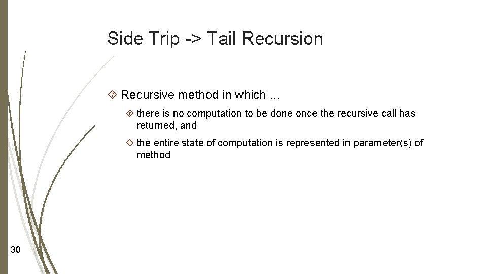
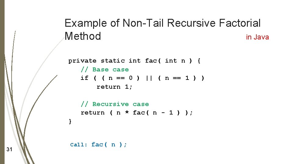
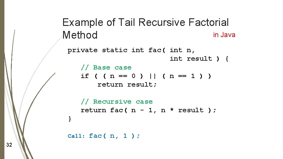
Side Trip -> Tail Recursion Recursive method in which … there is no computation to be done once the recursive call has returned, and the entire state of computation is represented in parameter(s) of method 30

Example of Non-Tail Recursive Factorial in Java Method private static int fac( int n ) { // Base case if ( ( n == 0 ) || ( n == 1 ) ) return 1; // Recursive case return ( n * fac( n - 1 ) ); } 31 Call: fac( n );

Example of Tail Recursive Factorial in Java Method private static int fac( int n, int result ) { // Base case if ( ( n == 0 ) || ( n == 1 ) ) return result; // Recursive case return fac( n - 1, n * result ); } Call: 32 fac( n, 1 );

Advantages of Tail Recursion - 1 Can be transformed into equivalent iterative method by replacing recursive method call using a loop 33

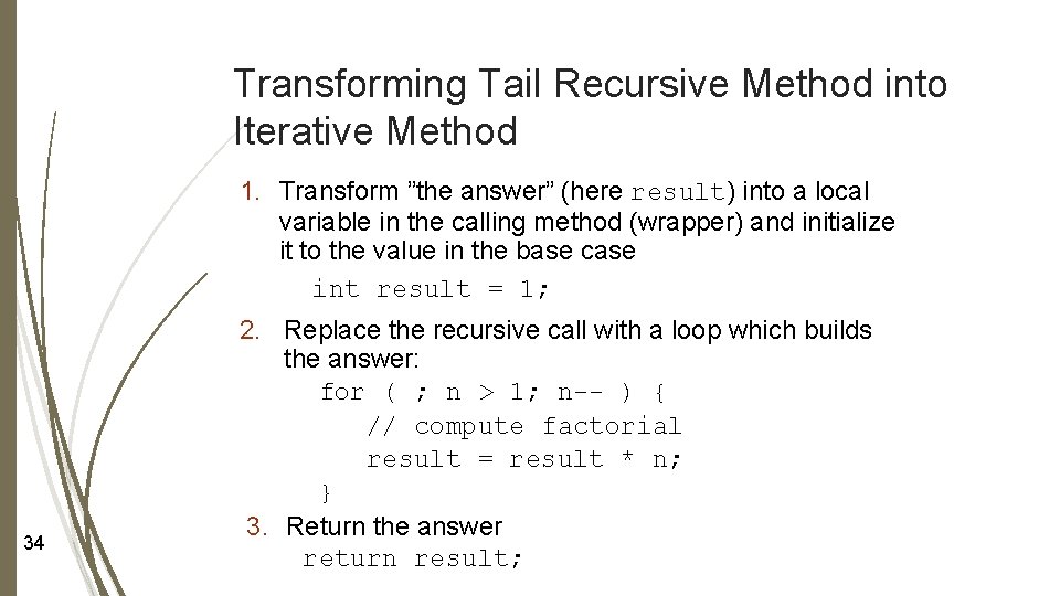
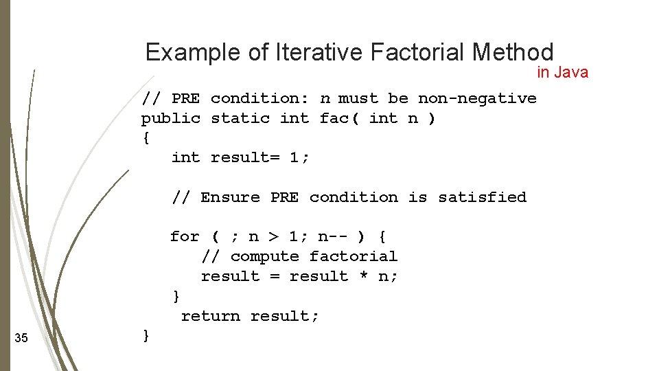
Transforming Tail Recursive Method into Iterative Method 1. Transform ”the answer” (here result) into a local variable in the calling method (wrapper) and initialize it to the value in the base case int result = 1; 34 2. Replace the recursive call with a loop which builds the answer: for ( ; n > 1; n-- ) { // compute factorial result = result * n; } 3. Return the answer return result;

Example of Iterative Factorial Method in Java // PRE condition: n must be non-negative public static int fac( int n ) { int result= 1; // Ensure PRE condition is satisfied for ( ; n > 1; n-- ) { // compute factorial result = result * n; } return result; 35 }

Advantages of Tail Recursion - 2 Tail Recursion Optimization A compiler may recognize “tail recursion” and optimize the code by replacing the calling statement with the called method (with some modifications), so that instead of nesting the stack deeper, the current stack frame is reused when the code execute, i. e. , no other stack frame than the first one is needed This allows a software developer to write (tail) recursive methods without worrying about space inefficiency during execution The tail recursive code is then as efficient as iterative version Reference: http: //c 2. com/cgi/wiki? Tail. Recursion & http: //en. wikipedia. org/wiki/Tail_call 36

Example of Improvement 4 37 // For complete running code, see http: //code. geeksforgeeks. org/LHxw. Pk