CMPE 371 Analysis of Algorithms FALL 2020 2021

CMPE 371 Analysis of Algorithms FALL 2020 -2021 Lecture 5

Analysis of Algorithms Part II: Algorithm Design Techniques • Programming paradigms • Brute force approach • Divide and conquer • Dynamic programming: • matrix chain multiplication problem • longest common subsequence problem • rod cuting problem • Greedy algorithms: • activity selection problem • fractional knapsack problem

Programming paradigms programming paradigm = general approach to algorithm design = general philosophy for solving a problem there are different ways of solving a problem several possible programming paradigms to solve the same problem a programming paradigm may be adapted to a certain problem and not to another

Brute Force A straightforward approach, usually based directly on the problem’s statement and definitions of the concepts involved Examples: 1. Computing an (a > 0, n a nonnegative integer) 2. Computing n! 3. Multiplying two matrices 4. Searching for a key of a given value in a list

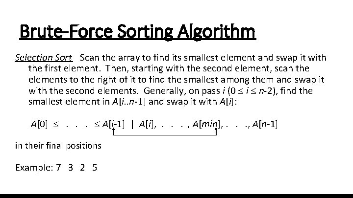
Brute-Force Sorting Algorithm Selection Sort Scan the array to find its smallest element and swap it with the first element. Then, starting with the second element, scan the elements to the right of it to find the smallest among them and swap it with the second elements. Generally, on pass i (0 i n-2), find the smallest element in A[i. . n-1] and swap it with A[i]: A[0] . . . A[i-1] | A[i], . . . , A[min], . . . , A[n-1] in their final positions Example: 7 3 2 5

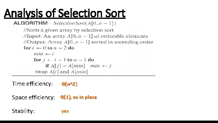
Analysis of Selection Sort Time efficiency: Θ(n^2 ) Space efficiency: Θ(1), so in place Stability: yes

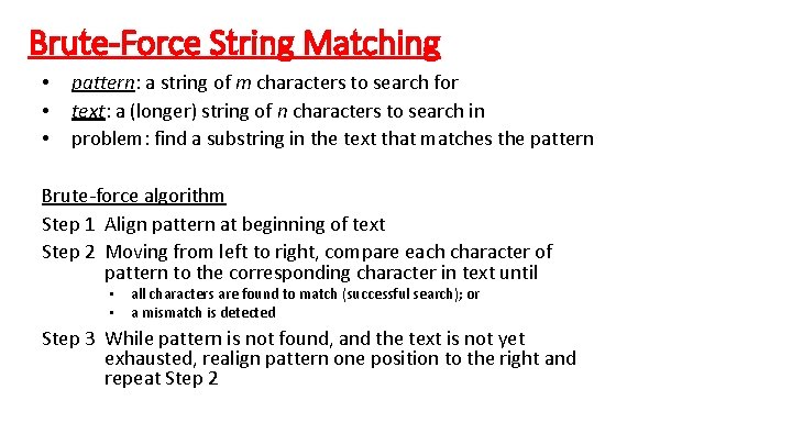
Brute-Force String Matching • • • pattern: a string of m characters to search for text: a (longer) string of n characters to search in problem: find a substring in the text that matches the pattern Brute-force algorithm Step 1 Align pattern at beginning of text Step 2 Moving from left to right, compare each character of pattern to the corresponding character in text until • • all characters are found to match (successful search); or a mismatch is detected Step 3 While pattern is not found, and the text is not yet exhausted, realign pattern one position to the right and repeat Step 2

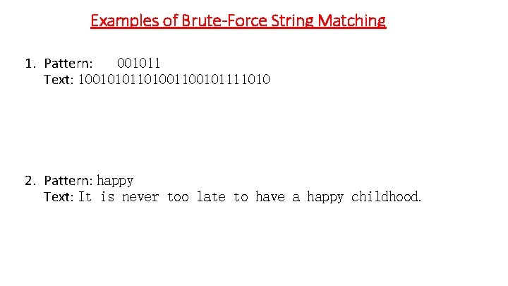
Examples of Brute-Force String Matching 1. Pattern: 001011 Text: 1001010110100101111010 2. Pattern: happy Text: It is never too late to have a happy childhood.

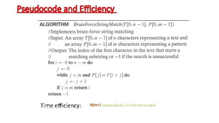
Pseudocode and Efficiency Time efficiency: Θ(mn) comparisons (in the worst case)

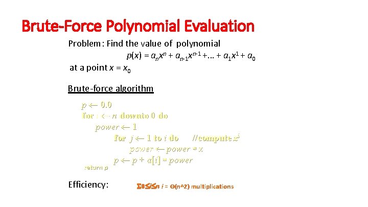
Brute-Force Polynomial Evaluation Problem: Find the value of polynomial p(x) = anxn + an-1 xn-1 +… + a 1 x 1 + a 0 at a point x = x 0 Brute-force algorithm p 0. 0 for i n downto 0 do power 1 for j 1 to i do //compute xi power x p p + a[i] power return p Efficiency: 0 i n i = Θ(n^2) multiplications

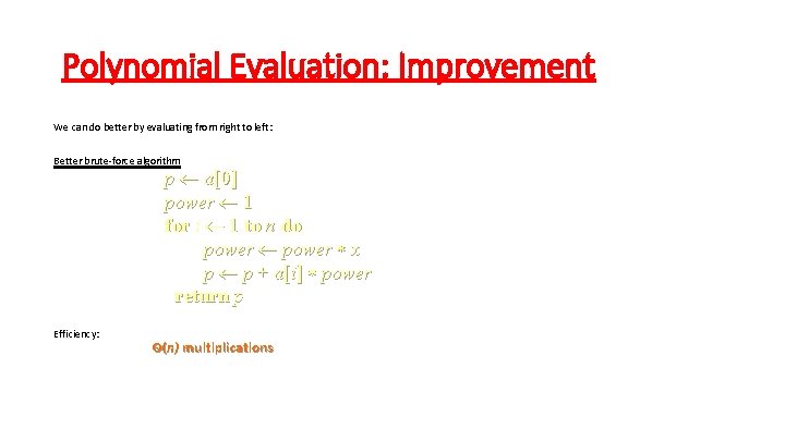
Polynomial Evaluation: Improvement We can do better by evaluating from right to left: Better brute-force algorithm p a[0] power 1 for i 1 to n do power x p p + a[i] power return p Efficiency: Θ(n) multiplications

Brute-Force Strengths and Weaknesses • Strengths • wide applicability • simplicity • yields reasonable algorithms for some important problems (e. g. , matrix multiplication, sorting, searching, string matching) • Weaknesses • rarely yields efficient algorithms • some brute-force algorithms are unacceptably slow • not as constructive as some other design techniques

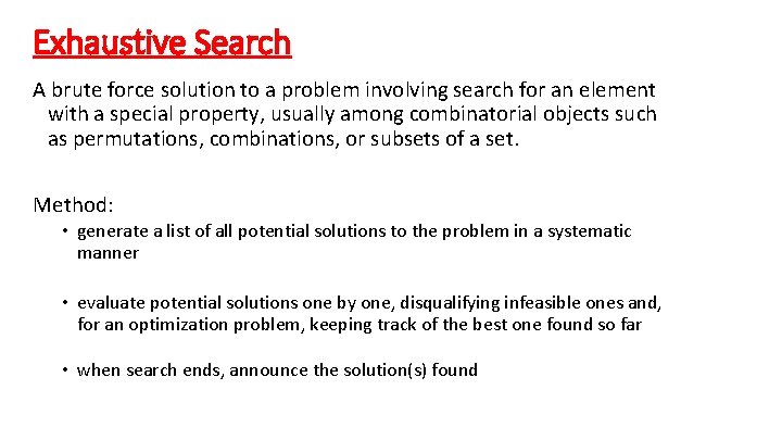
Exhaustive Search A brute force solution to a problem involving search for an element with a special property, usually among combinatorial objects such as permutations, combinations, or subsets of a set. Method: • generate a list of all potential solutions to the problem in a systematic manner • evaluate potential solutions one by one, disqualifying infeasible ones and, for an optimization problem, keeping track of the best one found so far • when search ends, announce the solution(s) found

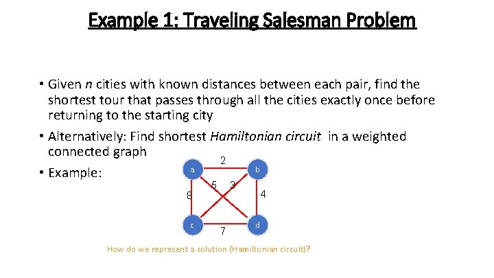
Example 1: Traveling Salesman Problem • Given n cities with known distances between each pair, find the shortest tour that passes through all the cities exactly once before returning to the starting city • Alternatively: Find shortest Hamiltonian circuit in a weighted connected graph 2 a b • Example: 8 c 5 3 7 4 d How do we represent a solution (Hamiltonian circuit)?

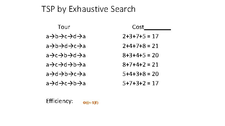
TSP by Exhaustive Search Tour a→b→c→d→a a→b→d→c→a a→c→b→d→a a→c→d→b→a a→d→b→c→a a→d→c→b→a Efficiency: Θ((n-1)!) Cost 2+3+7+5 = 17 2+4+7+8 = 21 8+3+4+5 = 20 8+7+4+2 = 21 5+4+3+8 = 20 5+7+3+2 = 17

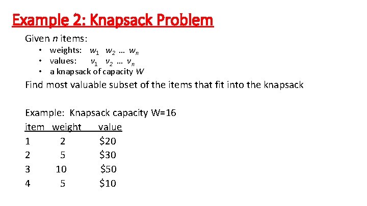
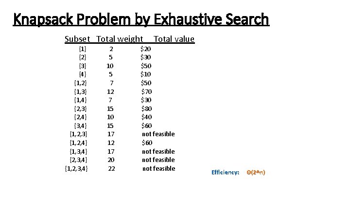
Example 2: Knapsack Problem Given n items: • weights: w 1 w 2 … wn • values: v 1 v 2 … vn • a knapsack of capacity W Find most valuable subset of the items that fit into the knapsack Example: Knapsack capacity W=16 item weight value 1 2 $20 2 5 $30 3 10 $50 4 5 $10

Knapsack Problem by Exhaustive Search Subset Total weight {1} {2} {3} {4} {1, 2} {1, 3} {1, 4} {2, 3} {2, 4} {3, 4} {1, 2, 3} {1, 2, 4} {1, 3, 4} {2, 3, 4} {1, 2, 3, 4} 2 5 10 5 7 12 7 15 10 15 17 12 17 20 22 Total value $20 $30 $50 $10 $50 $70 $30 $80 $40 $60 not feasible Efficiency: Θ(2^n)

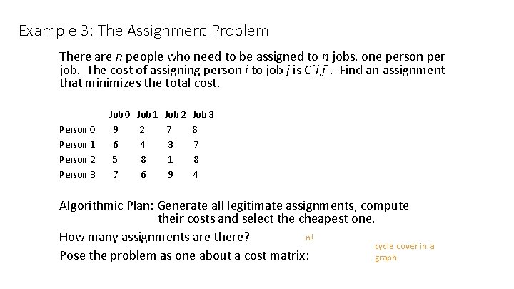
Example 3: The Assignment Problem There are n people who need to be assigned to n jobs, one person per job. The cost of assigning person i to job j is C[i, j]. Find an assignment that minimizes the total cost. Person 0 Person 1 Person 2 Person 3 Job 0 Job 1 Job 2 9 2 7 6 4 3 5 8 1 7 6 9 Job 3 8 7 8 4 Algorithmic Plan: Generate all legitimate assignments, compute their costs and select the cheapest one. n! How many assignments are there? cycle cover in a Pose the problem as one about a cost matrix: graph

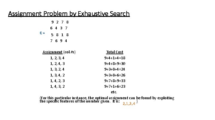
Assignment Problem by Exhaustive Search C= 9 2 7 8 6 4 3 7 5 8 1 8 7 6 9 4 Assignment (col. #s) 1, 2, 3, 4 1, 2, 4, 3 1, 3, 2, 4 1, 3, 4, 2 1, 4, 2, 3 1, 4, 3, 2 Total Cost 9+4+1+4=18 9+4+8+9=30 9+3+8+4=24 9+3+8+6=26 9+7+8+9=33 9+7+1+6=23 etc. (For this particular instance, the optimal assignment can be found by exploiting the specific features of the number given. It is: ) 2, 1, 3, 4

Final Comments on Exhaustive Search • Exhaustive-search algorithms run in a realistic amount of time only on very small instances • In some cases, there are much better alternatives! • • Euler circuits shortest paths minimum spanning tree assignment problem • In many cases, exhaustive search or its variation is the only known way to get exact solution

Divide-and-Conquer

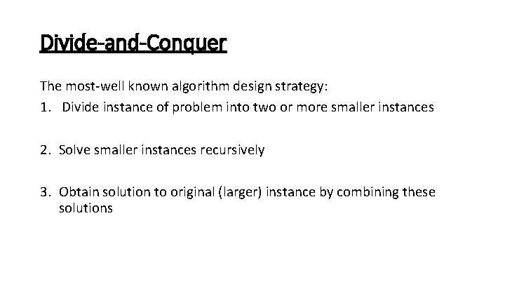
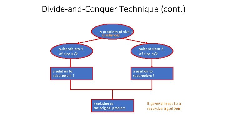
Divide-and-Conquer The most-well known algorithm design strategy: 1. Divide instance of problem into two or more smaller instances 2. Solve smaller instances recursively 3. Obtain solution to original (larger) instance by combining these solutions

Divide-and-Conquer Technique (cont. ) a problem of size n (instance) subproblem 1 of size n/2 subproblem 2 of size n/2 a solution to subproblem 1 a solution to subproblem 2 a solution to the original problem It general leads to a recursive algorithm!

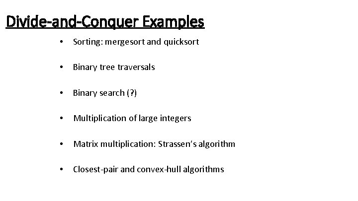
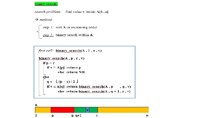
Divide-and-Conquer Examples • Sorting: mergesort and quicksort • Binary tree traversals • Binary search (? ) • Multiplication of large integers • Matrix multiplication: Strassen’s algorithm • Closest-pair and convex-hull algorithms

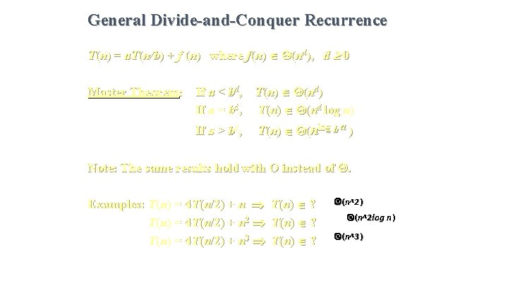
General Divide-and-Conquer Recurrence T(n) = a. T(n/b) + f (n) where f(n) (nd), d 0 Master Theorem: If a < bd, T(n) (nd) If a = bd, T(n) (nd log n) If a > bd, T(n) (nlog b a ) Note: The same results hold with O instead of . Examples: T(n) = 4 T(n/2) + n 2 T(n) = 4 T(n/2) + n 3 T (n ) ? (n^2 ) (n^2 log n ) (n^3 )

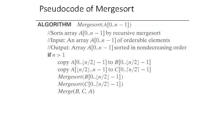
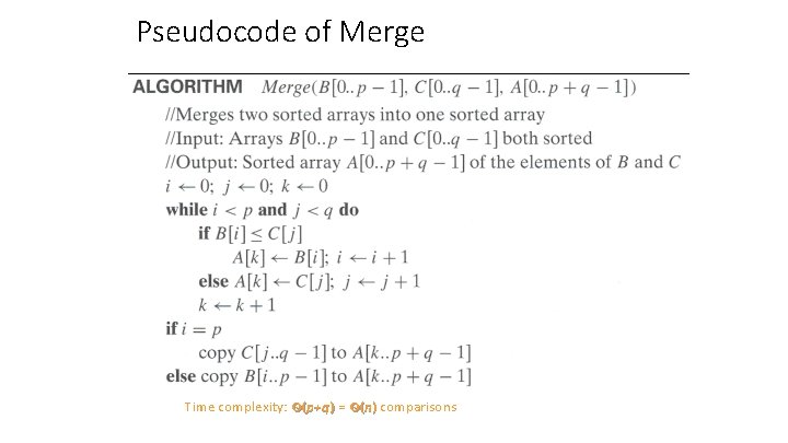
Mergesort • Split array A[0. . n-1] into about equal halves and make copies of each half in arrays B and C • Sort arrays B and C recursively • Merge sorted arrays B and C into array A as follows: • Repeat the following until no elements remain in one of the arrays: • compare the first elements in the remaining unprocessed portions of the arrays • copy the smaller of the two into A, while incrementing the index indicating the unprocessed portion of that array • Once all elements in one of the arrays are processed, copy the remaining unprocessed elements from the other array into A.

Pseudocode of Mergesort

Pseudocode of Merge Time complexity: Θ(p+q ) = Θ(n) comparisons

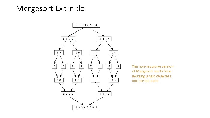
Mergesort Example The non-recursive version of Mergesort starts from merging single elements into sorted pairs.

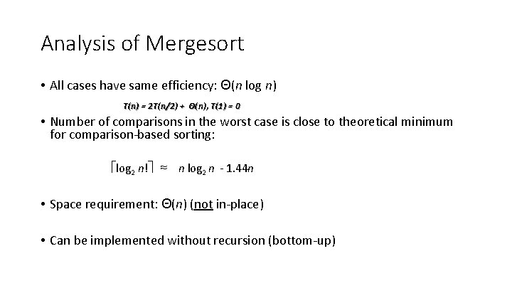
Analysis of Mergesort • All cases have same efficiency: Θ(n log n) T(n) = 2 T(n/2) + Θ(n), T(1) = 0 • Number of comparisons in the worst case is close to theoretical minimum for comparison-based sorting: log 2 n! ≈ n log 2 n - 1. 44 n • Space requirement: Θ(n) (not in-place) • Can be implemented without recursion (bottom-up)