CMPE 140 Intro To Computing for Economics and

CMPE 140 Intro. To Computing for Economics and Management Fall 2015 9. Input/Output

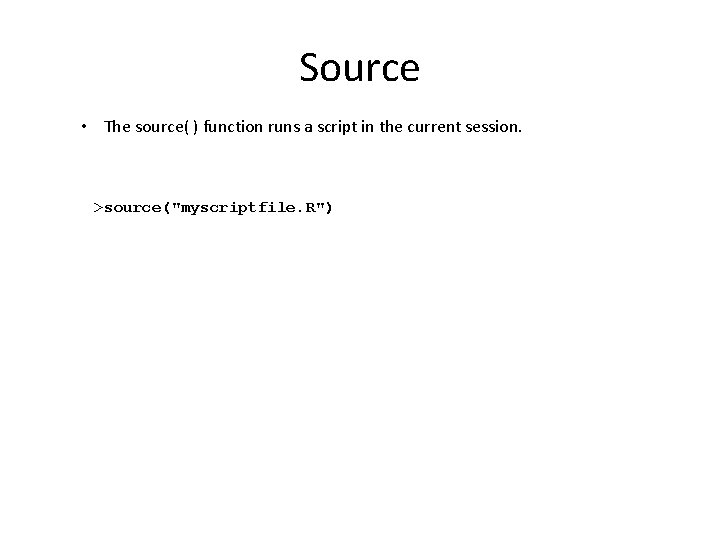
Source • The source( ) function runs a script in the current session. >source("myscriptfile. R")

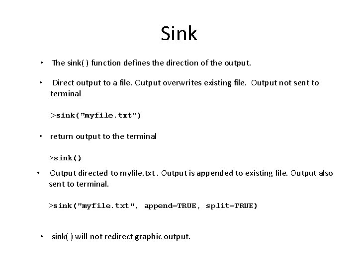
Sink • The sink( ) function defines the direction of the output. • Direct output to a file. Output overwrites existing file. Output not sent to terminal >sink("myfile. txt”) • return output to the terminal >sink() • Output directed to myfile. txt. Output is appended to existing file. Output also sent to terminal. >sink("myfile. txt", append=TRUE, split=TRUE) • sink( ) will not redirect graphic output.

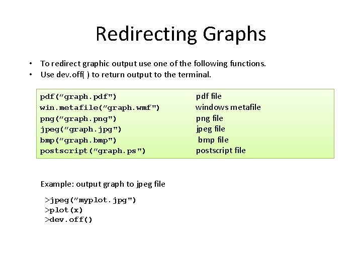
Redirecting Graphs • To redirect graphic output use one of the following functions. • Use dev. off( ) to return output to the terminal. pdf(”graph. pdf") win. metafile(”graph. wmf") png(”graph. png") jpeg(”graph. jpg") bmp(”graph. bmp") postscript(”graph. ps") Example: output graph to jpeg file >jpeg(”myplot. jpg") >plot(x) >dev. off() pdf file windows metafile png file jpeg file bmp file postscript file

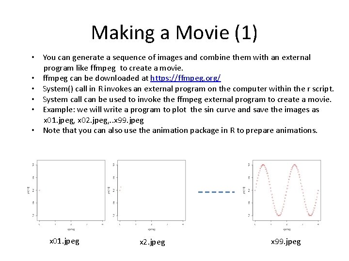
Making a Movie (1) • You can generate a sequence of images and combine them with an external program like ffmpeg to create a movie. • ffmpeg can be downloaded at https: //ffmpeg. org/ • System() call in R invokes an external program on the computer within the r script. • System call can be used to invoke the ffmpeg external program to create a movie. • Example: we will write a program to plot the sin curve and save the images as x 01. jpeg, x 02. jpeg, . . x 99. jpeg • Note that you can also use the animation package in R to prepare animations. x 01. jpeg x 2. jpeg x 99. jpeg

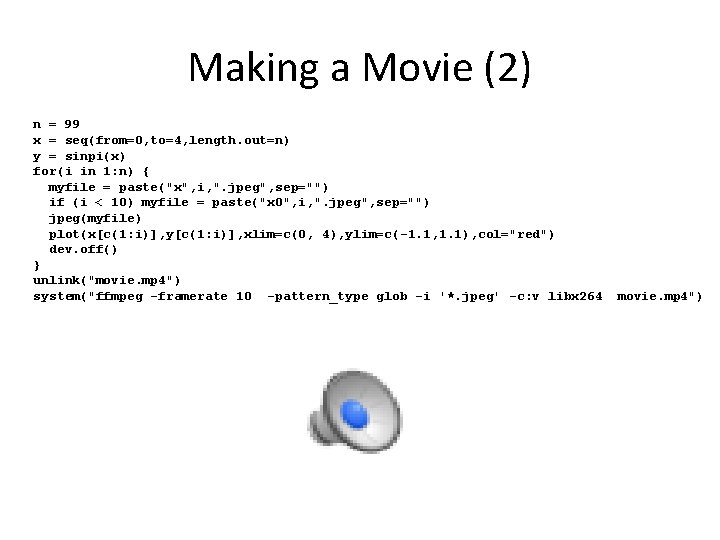
Making a Movie (2) n = 99 x = seq(from=0, to=4, length. out=n) y = sinpi(x) for(i in 1: n) { myfile = paste("x", i, ". jpeg", sep="") if (i < 10) myfile = paste("x 0", i, ". jpeg", sep="") jpeg(myfile) plot(x[c(1: i)], y[c(1: i)], xlim=c(0, 4), ylim=c(-1. 1, 1. 1), col="red") dev. off() } unlink("movie. mp 4") system("ffmpeg -framerate 10 -pattern_type glob -i '*. jpeg' -c: v libx 264 movie. mp 4")

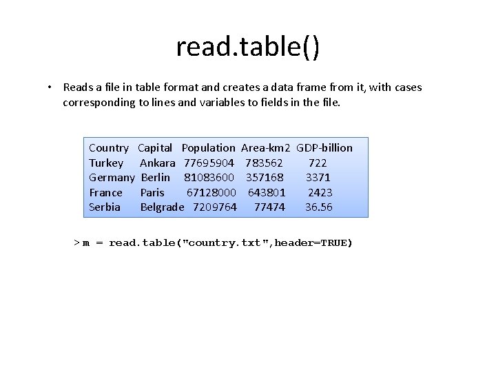
read. table() • Reads a file in table format and creates a data frame from it, with cases corresponding to lines and variables to fields in the file. Country Capital Population Turkey Ankara 77695904 Germany Berlin 81083600 France Paris 67128000 Serbia Belgrade 7209764 Area-km 2 GDP-billion 783562 722 357168 3371 643801 2423 77474 36. 56 > m = read. table("country. txt", header=TRUE)

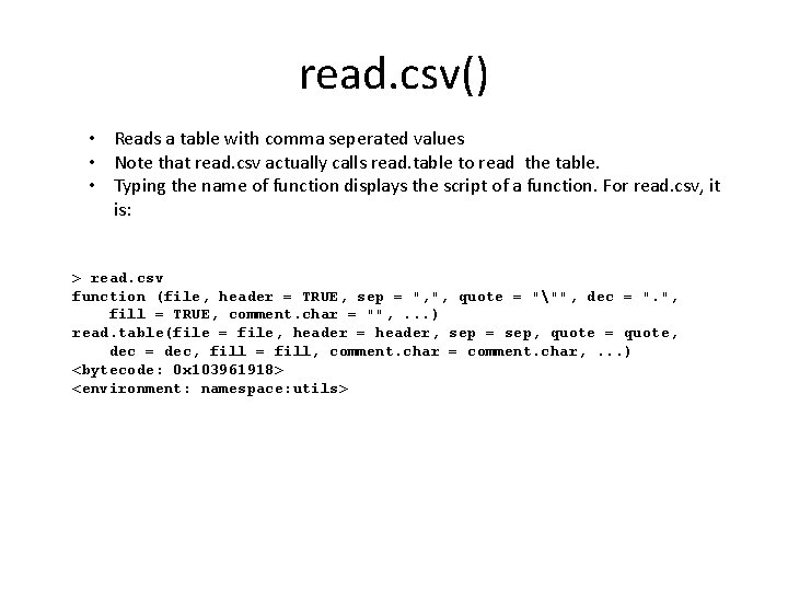
read. csv() • Reads a table with comma seperated values • Note that read. csv actually calls read. table to read the table. • Typing the name of function displays the script of a function. For read. csv, it is: > read. csv function (file, header = TRUE, sep = ", ", quote = """, dec = ". ", fill = TRUE, comment. char = "", . . . ) read. table(file = file, header = header, sep = sep, quote = quote, dec = dec, fill = fill, comment. char = comment. char, . . . ) <bytecode: 0 x 103961918> <environment: namespace: utils>

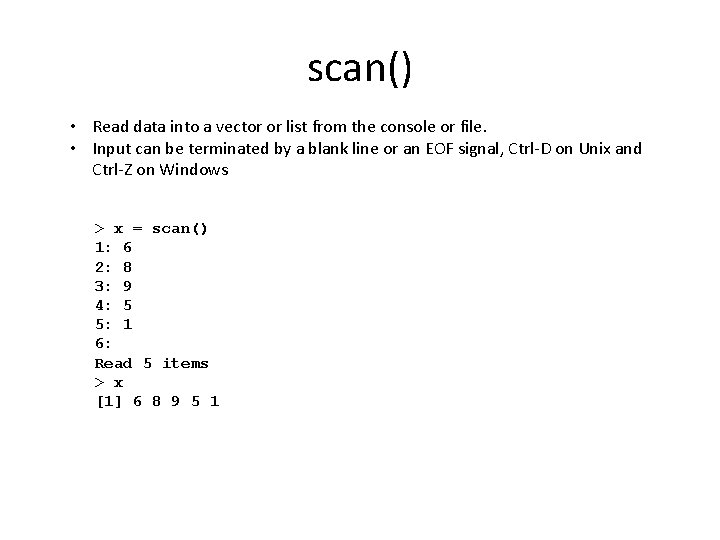
scan() • Read data into a vector or list from the console or file. • Input can be terminated by a blank line or an EOF signal, Ctrl-D on Unix and Ctrl-Z on Windows > x = scan() 1: 6 2: 8 3: 9 4: 5 5: 1 6: Read 5 items > x [1] 6 8 9 5 1

Reading Data from Internet JSON Format (1) • JSON, (Java. Script Object Notation), is an open standard format that uses humanreadable text to transmit data objects consisting of attribute–value pairs. • It is the primary data format used for asynchronous browser/server communication. • On the Internet, web server API (application programming interface) usually return data in JSON format. • Install jsonlite package to read data from the Internet in JSON format. • API examples: http: //fixer. io/ Fixer. io is a free JSON API for current and historical foreign exchange rates published by the European Central Bank. https: //www. bitstamp. net/api/ bitcoin trading data (bids, asks, averages etc).

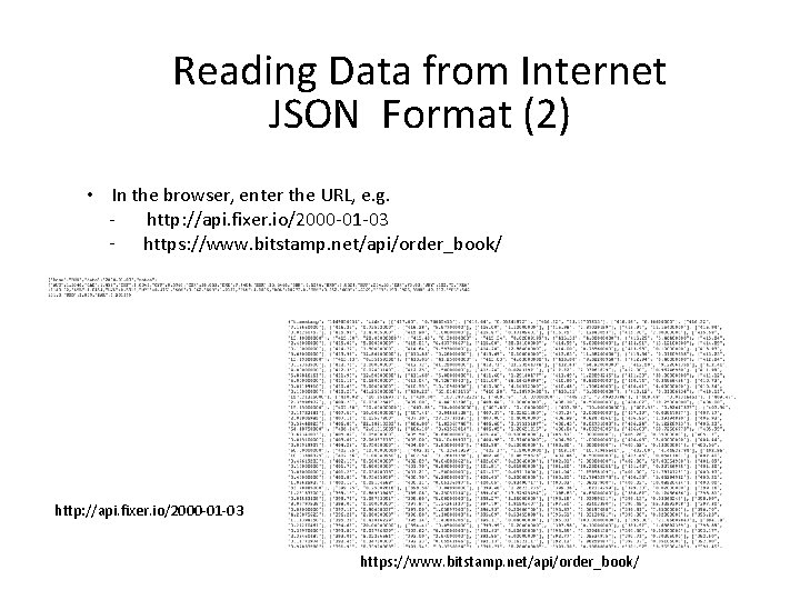
Reading Data from Internet JSON Format (2) • In the browser, enter the URL, e. g. http: //api. fixer. io/2000 -01 -03 - https: //www. bitstamp. net/api/order_book/ http: //api. fixer. io/2000 -01 -03 https: //www. bitstamp. net/api/order_book/

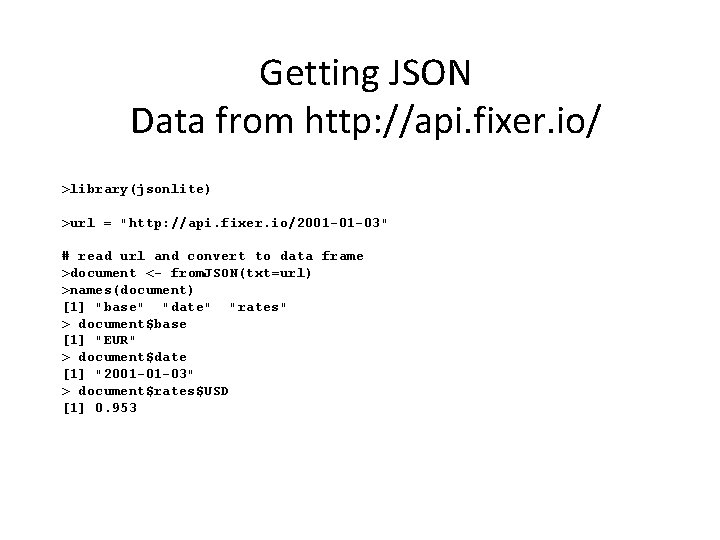
Getting JSON Data from http: //api. fixer. io/ >library(jsonlite) >url = "http: //api. fixer. io/2001 -01 -03" # read url and convert to data frame >document <- from. JSON(txt=url) >names(document) [1] "base" "date" "rates" > document$base [1] "EUR" > document$date [1] "2001 -01 -03" > document$rates$USD [1] 0. 953

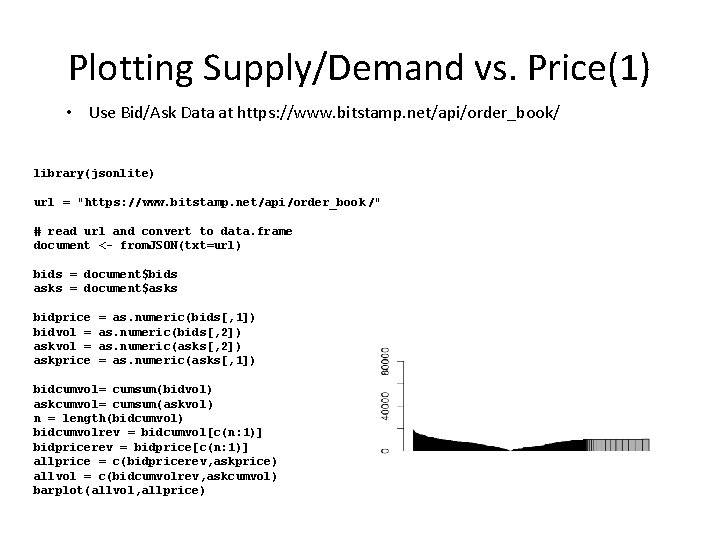
Plotting Supply/Demand vs. Price(1) • Use Bid/Ask Data at https: //www. bitstamp. net/api/order_book/ library(jsonlite) url = "https: //www. bitstamp. net/api/order_book /" # read url and convert to data. frame document <- from. JSON(txt=url) bids = document$bids asks = document$asks bidprice bidvol = askprice = as. numeric(bids[, 1]) as. numeric(bids[, 2]) as. numeric(asks[, 2]) = as. numeric(asks[, 1]) bidcumvol= cumsum(bidvol) askcumvol= cumsum(askvol ) n = length(bidcumvol) bidcumvolrev = bidcumvol[c(n: 1)] bidpricerev = bidprice[c(n: 1)] allprice = c(bidpricerev, askprice) allvol = c(bidcumvolrev, askcumvol) barplot(allvol, allprice)

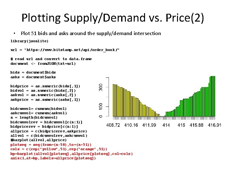
Plotting Supply/Demand vs. Price(2) • Plot 51 bids and asks around the supply/demand intersection library(jsonlite) url = "https: //www. bitstamp. net/api/order_book /" # read url and convert to data. frame document <- from. JSON(txt=url) bids = document$bids asks = document$asks bidprice bidvol = askprice = as. numeric(bids[, 1]) as. numeric(bids[, 2]) as. numeric(asks[, 2] ) = as. numeric(asks[, 1]) bidcumvol= cumsum(bidvol) askcumvol= cumsum(askvol ) n = length(bidcumvol) bidcumvolrev = bidcumvol[c(n: 1)] bidpricerev = bidprice[c(n: 1)] allprice = c(bidpricerev, askprice) allvol = c(bidcumvolrev, askcumvol ) #barplot(allvol, allprice) plotseq = seq(from=(n-50), to=(n+51)) cols = c(rep("yellow", 51), rep("orange", 51)) bp=barplot(allvol[plotseq], allprice[plotseq], col=cols ) axis(1, at=bp, labels=allprice[plotseq])