Clustering Wei Wang Outline What is clustering Partitioning

Clustering Wei Wang

Outline • • What is clustering Partitioning methods Hierarchical methods Density-based methods Grid-based methods Model-based clustering methods Outlier analysis

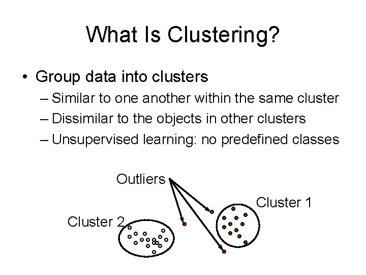
What Is Clustering? • Group data into clusters – Similar to one another within the same cluster – Dissimilar to the objects in other clusters – Unsupervised learning: no predefined classes Outliers Cluster 1 Cluster 2

Application Examples • A stand-alone tool: explore data distribution • A preprocessing step for other algorithms • Pattern recognition, spatial data analysis, image processing, market research, WWW, … – Cluster documents – Cluster web log data to discover groups of similar access patterns

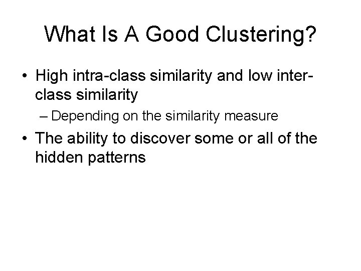
What Is A Good Clustering? • High intra-class similarity and low interclass similarity – Depending on the similarity measure • The ability to discover some or all of the hidden patterns

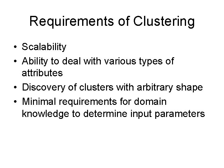
Requirements of Clustering • Scalability • Ability to deal with various types of attributes • Discovery of clusters with arbitrary shape • Minimal requirements for domain knowledge to determine input parameters

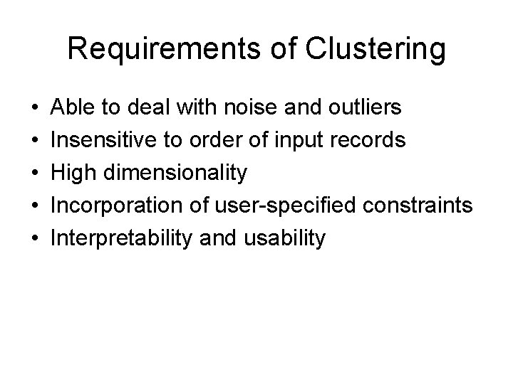
Requirements of Clustering • • • Able to deal with noise and outliers Insensitive to order of input records High dimensionality Incorporation of user-specified constraints Interpretability and usability

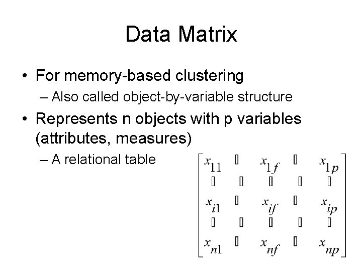
Data Matrix • For memory-based clustering – Also called object-by-variable structure • Represents n objects with p variables (attributes, measures) – A relational table

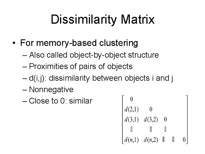
Dissimilarity Matrix • For memory-based clustering – Also called object-by-object structure – Proximities of pairs of objects – d(i, j): dissimilarity between objects i and j – Nonnegative – Close to 0: similar

How Good Is A Clustering? • Dissimilarity/similarity depends on distance function – Different applications have different functions • Judgment of clustering quality is typically highly subjective

Types of Data in Clustering • • Interval-scaled variables Binary variables Nominal, ordinal, and ratio variables Variables of mixed types

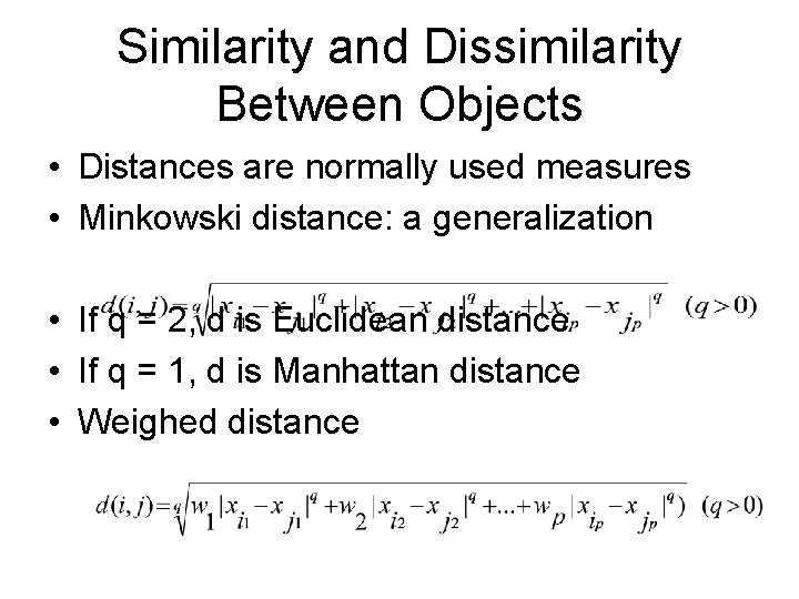
Similarity and Dissimilarity Between Objects • Distances are normally used measures • Minkowski distance: a generalization • If q = 2, d is Euclidean distance • If q = 1, d is Manhattan distance • Weighed distance

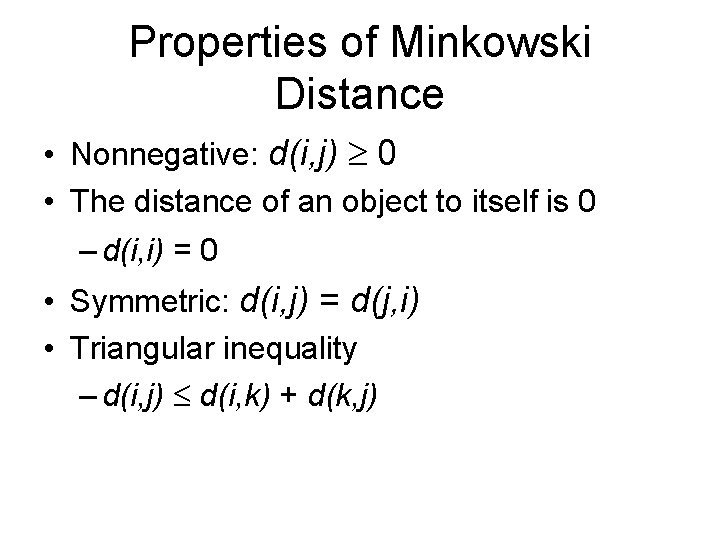
Properties of Minkowski Distance • Nonnegative: d(i, j) 0 • The distance of an object to itself is 0 – d(i, i) = 0 • Symmetric: d(i, j) = d(j, i) • Triangular inequality – d(i, j) d(i, k) + d(k, j)

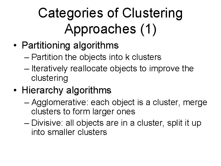
Categories of Clustering Approaches (1) • Partitioning algorithms – Partition the objects into k clusters – Iteratively reallocate objects to improve the clustering • Hierarchy algorithms – Agglomerative: each object is a cluster, merge clusters to form larger ones – Divisive: all objects are in a cluster, split it up into smaller clusters

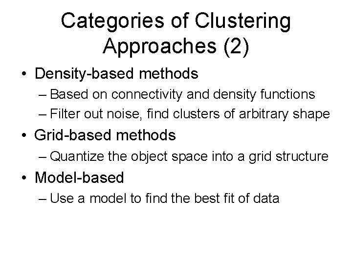
Categories of Clustering Approaches (2) • Density-based methods – Based on connectivity and density functions – Filter out noise, find clusters of arbitrary shape • Grid-based methods – Quantize the object space into a grid structure • Model-based – Use a model to find the best fit of data

Partitioning Algorithms: Basic Concepts • Partition n objects into k clusters – Optimize the chosen partitioning criterion • Global optimal: examine all partitions – (kn-(k-1)n-…-1) possible partitions, too expensive! • Heuristic methods: k-means and k-medoids – K-means: a cluster is represented by the center – K-medoids or PAM (partition around medoids): each cluster is represented by one of the objects in the cluster

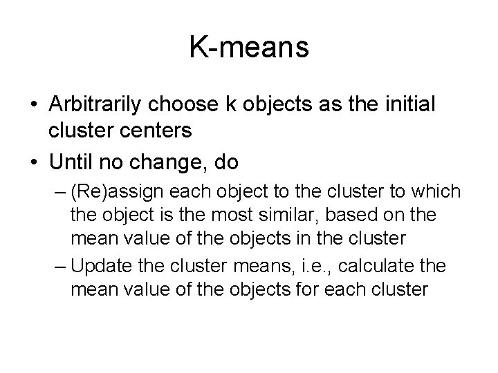
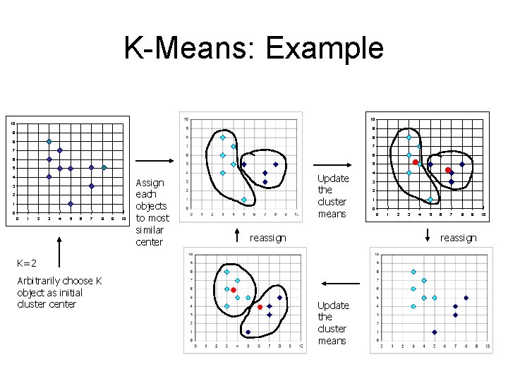
K-means • Arbitrarily choose k objects as the initial cluster centers • Until no change, do – (Re)assign each object to the cluster to which the object is the most similar, based on the mean value of the objects in the cluster – Update the cluster means, i. e. , calculate the mean value of the objects for each cluster

K-Means: Example 10 10 9 9 8 8 7 7 6 6 5 5 4 3 2 1 0 0 1 2 3 4 5 6 7 8 9 10 Assign each objects to most similar center Update the cluster means reassign 3 2 1 0 0 1 2 3 4 5 6 7 8 9 reassign K=2 Arbitrarily choose K object as initial cluster center 4 Update the cluster means 10

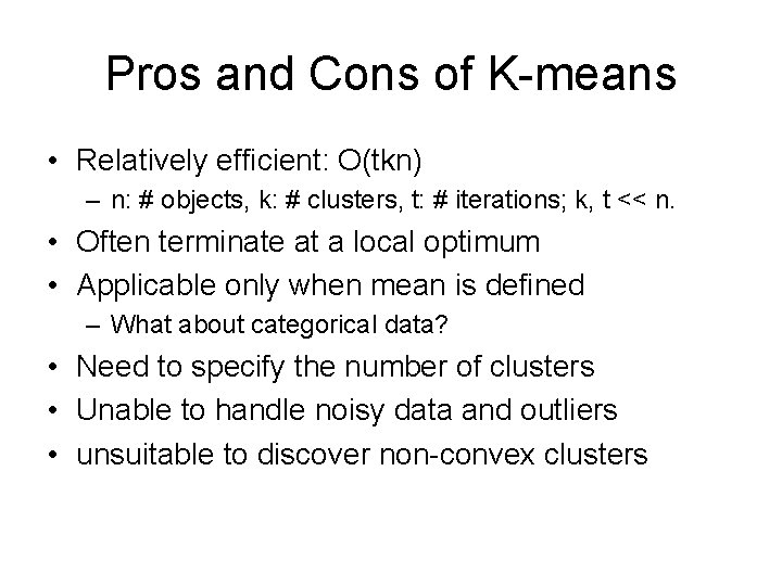
Pros and Cons of K-means • Relatively efficient: O(tkn) – n: # objects, k: # clusters, t: # iterations; k, t << n. • Often terminate at a local optimum • Applicable only when mean is defined – What about categorical data? • Need to specify the number of clusters • Unable to handle noisy data and outliers • unsuitable to discover non-convex clusters

Variations of the K-means • Aspects of variations – Selection of the initial k means – Dissimilarity calculations – Strategies to calculate cluster means • Handling categorical data: k-modes – Use mode instead of mean • Mode: the most frequent item(s) – A mixture of categorical and numerical data: kprototype method

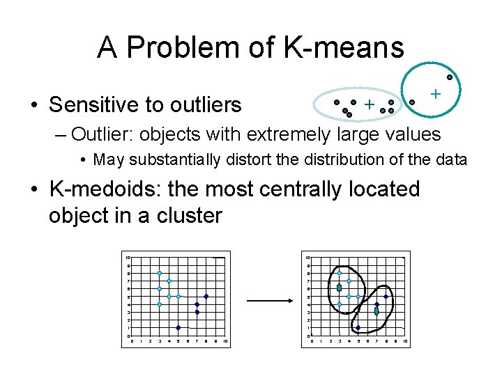
A Problem of K-means • Sensitive to outliers + + – Outlier: objects with extremely large values • May substantially distort the distribution of the data • K-medoids: the most centrally located object in a cluster 10 10 9 9 8 8 7 7 6 6 5 5 4 4 3 3 2 2 1 1 0 0 0 1 2 3 4 5 6 7 8 9 10

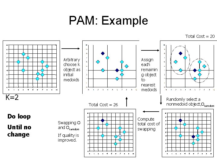
PAM: A K-medoids Method • PAM: partitioning around Medoids • Arbitrarily choose k objects as the initial medoids • Until no change, do – (Re)assign each object to the cluster to which the nearest medoid – Randomly select a non-medoid object o’, compute the total cost, S, of swapping medoid o with o’ – If S < 0 then swap o with o’ to form the new set of k medoids

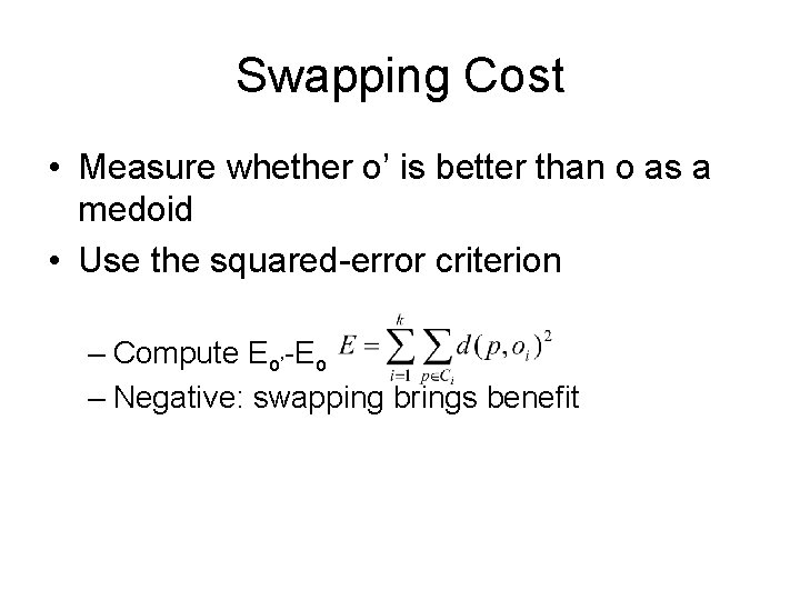
Swapping Cost • Measure whether o’ is better than o as a medoid • Use the squared-error criterion – Compute Eo’-Eo – Negative: swapping brings benefit

PAM: Example Total Cost = 20 10 9 8 Arbitrary choose k object as initial medoids 7 6 5 4 3 2 Assign each remainin g object to nearest medoids 1 0 0 1 2 3 4 5 6 7 8 9 10 K=2 Randomly select a nonmedoid object, Oramdom Total Cost = 26 Do loop Until no change 10 10 9 Swapping O and Oramdom If quality is improved. Compute total cost of swapping 8 7 6 9 8 7 6 5 5 4 4 3 3 2 2 1 1 0 0 0 1 2 3 4 5 6 7 8 9 10

Pros and Cons of PAM • PAM is more robust than k-means in the presence of noise and outliers – Medoids are less influenced by outliers • PAM is efficiently for small data sets but does not scale well for large data sets – O(k(n-k)2 ) for each iteration • Sampling based method: CLARA

CLARA (Clustering LARge Applications) • CLARA (Kaufmann and Rousseeuw in 1990) – Built in statistical analysis packages, such as S+ • Draw multiple samples of the data set, apply PAM on each sample, give the best clustering • Perform better than PAM in larger data sets • Efficiency depends on the sample size – A good clustering on samples may not be a good clustering of the whole data set

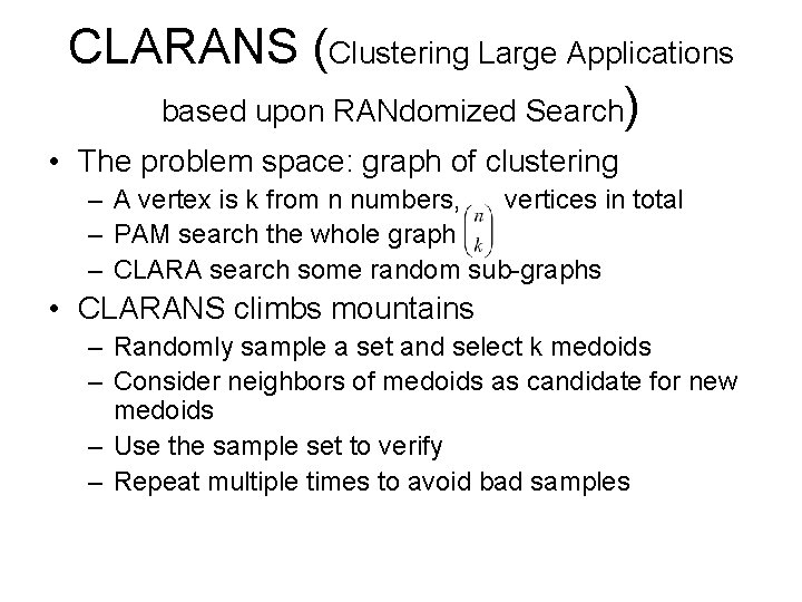
CLARANS (Clustering Large Applications based upon RANdomized Search) • The problem space: graph of clustering – A vertex is k from n numbers, vertices in total – PAM search the whole graph – CLARA search some random sub-graphs • CLARANS climbs mountains – Randomly sample a set and select k medoids – Consider neighbors of medoids as candidate for new medoids – Use the sample set to verify – Repeat multiple times to avoid bad samples