Clustering Mac Kay Chapter 20 Machine Learning Unsupervised

Clustering Mac. Kay - Chapter 20

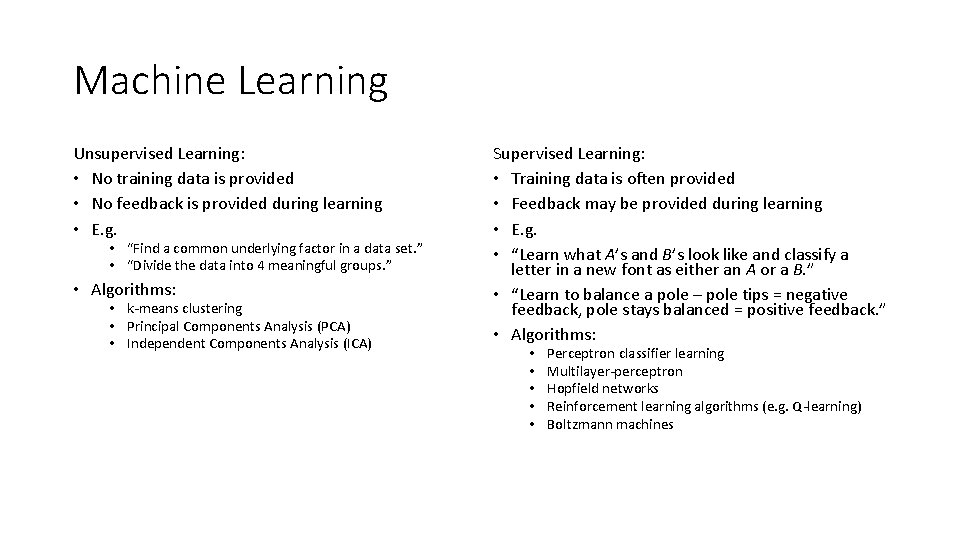
Machine Learning Unsupervised Learning: • No training data is provided • No feedback is provided during learning • E. g. • “Find a common underlying factor in a data set. ” • “Divide the data into 4 meaningful groups. ” • Algorithms: • k-means clustering • Principal Components Analysis (PCA) • Independent Components Analysis (ICA) Supervised Learning: • Training data is often provided • Feedback may be provided during learning • E. g. • “Learn what A’s and B’s look like and classify a letter in a new font as either an A or a B. ” • “Learn to balance a pole – pole tips = negative feedback, pole stays balanced = positive feedback. ” • Algorithms: • • • Perceptron classifier learning Multilayer-perceptron Hopfield networks Reinforcement learning algorithms (e. g. Q-learning) Boltzmann machines

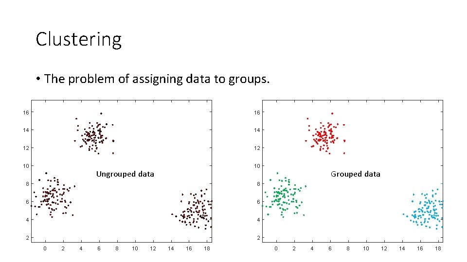
Clustering • The problem of assigning data to groups. 16 16 14 14 12 12 10 10 Ungrouped data 8 8 6 6 4 4 2 2 0 2 4 6 8 10 12 14 16 18 Grouped data 0 2 4 6 8 10 12 14 16 18

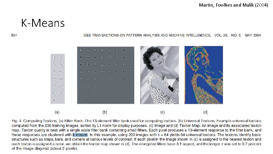
Martin, Fowlkes and Malik (2004) K-Means

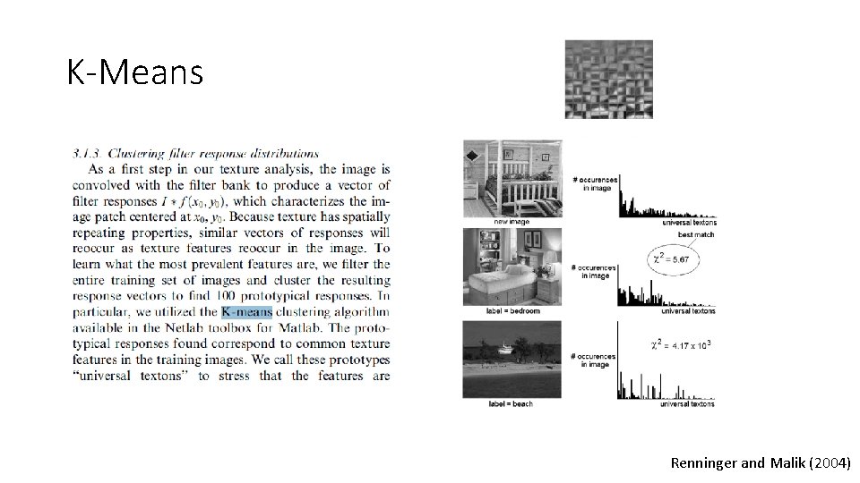
K-Means Renninger and Malik (2004)

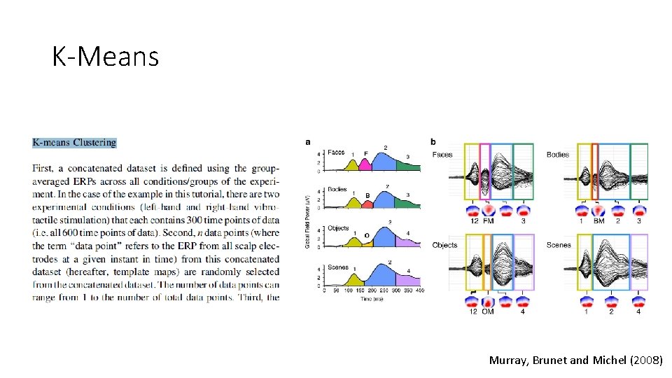
K-Means Murray, Brunet and Michel (2008)

K-Means

K-Means

K-Means

K-Means

K-Means

K-Means

K-Means

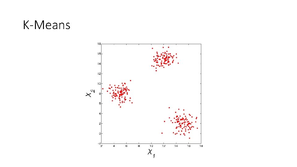
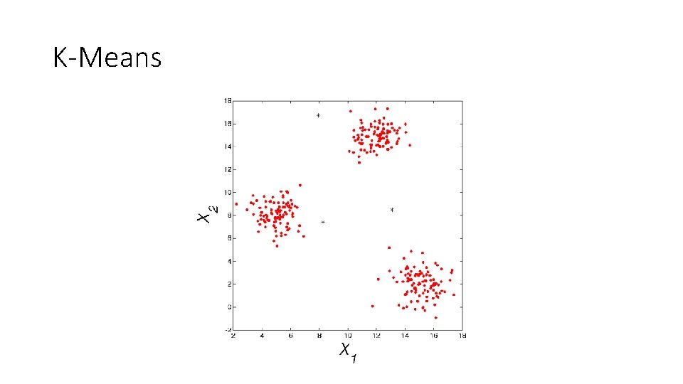
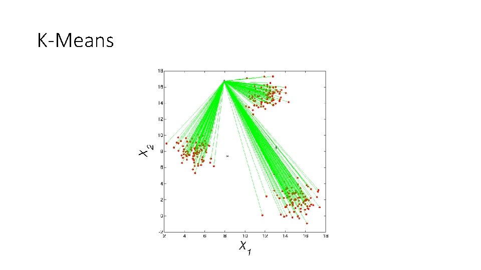
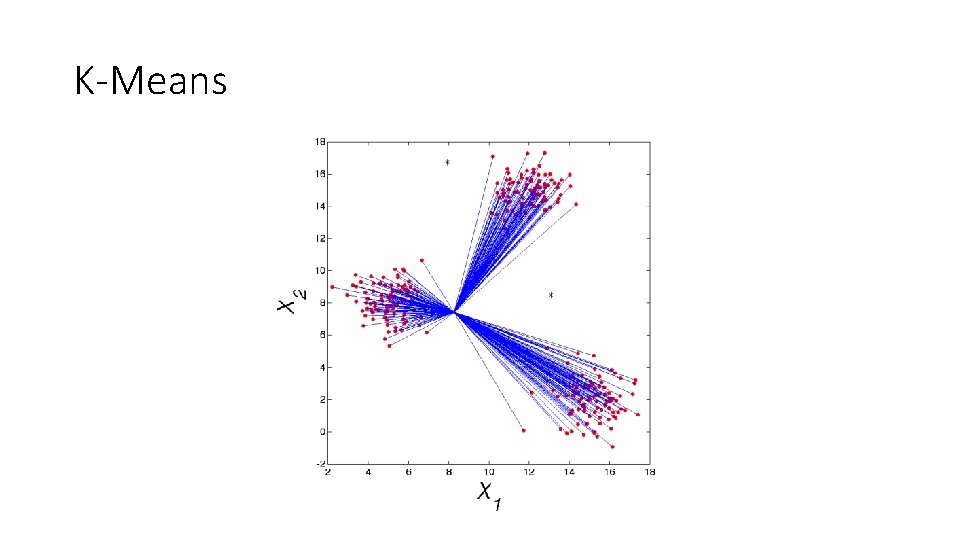
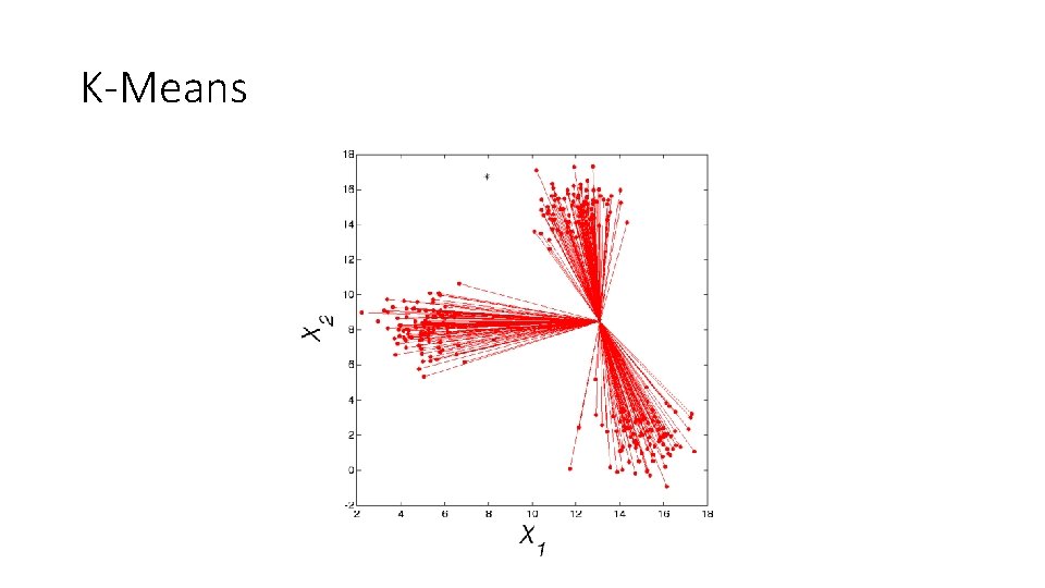
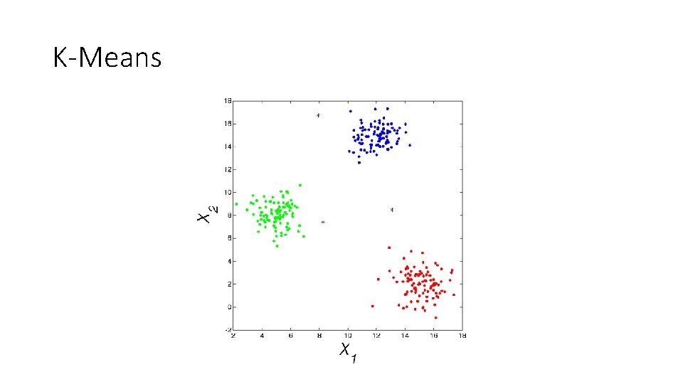
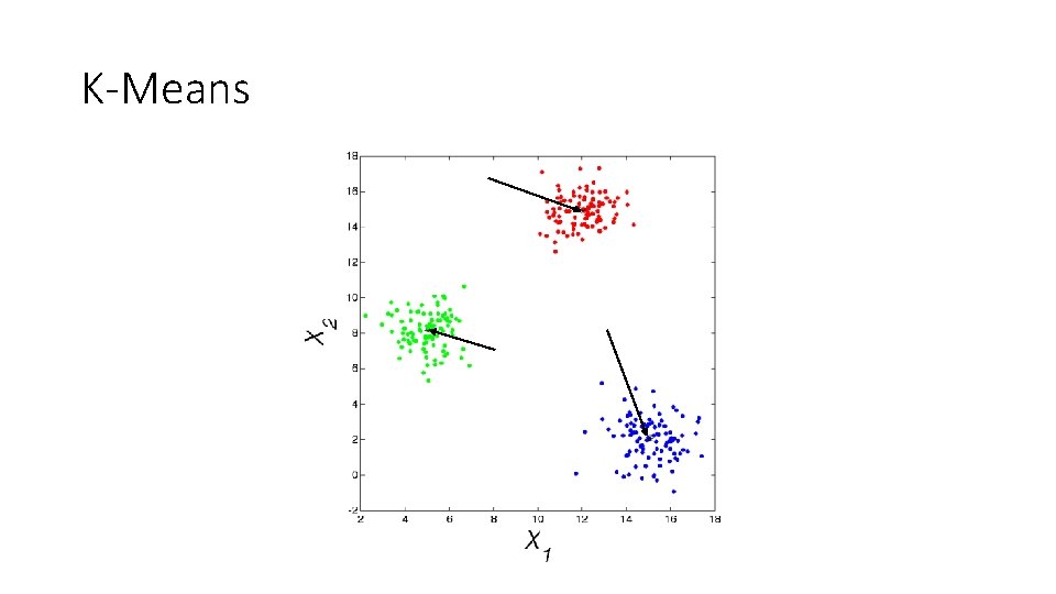
K-Means • The Algorithm • Randomly pick K-means. • Calculate the distance from each point to each mean. The mean that is closest to a given point wins that point. • Re-calculate each mean as the mean of the points it has just won. • Iterate until the total distance moved by all of the means is a very small number (like zero).

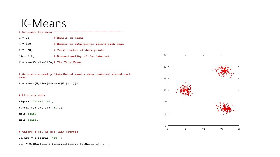
K-Means % Generate toy data --------------------K = 3; % Number of means n = 100; % Number of data points around each mean N = n*K; % Total number of data points dims = 2; % Dimensionality of the data set 25 M = rand(K, dims)*20; % The True Means 20 % Generate normally distributed random data centered around each mean 15 X = randn(N, dims)+repmat(M, [n 1]); 10 % Plot the data figure('Color', 'w'); 5 plot(X(: , 1), X(: , 2), 'r. '); axis equal; 0 axis square; -5 % Choose a colour for each cluster Col. Map = colormap('jet'); Col = Col. Map(round(linspace(1, size(Col. Map, 1), K)), : ); 0 5 10 15 20

K-Means % K means algorithm ---------------------% Initialize the K means m = rand(K, dims)*20; % Initialize distances matrix Dists = zeros(N, K); % Initialize the categories matrix Khat = zeros(N, 1); Keep. Going = true;

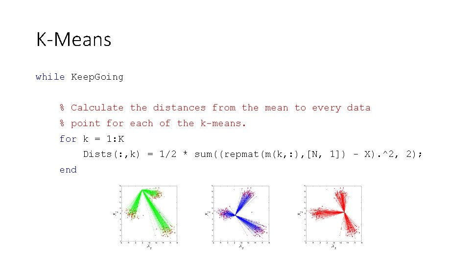
K-Means while Keep. Going % Calculate the distances from the mean to every data % point for each of the k-means. for k = 1: K Dists(: , k) = 1/2 * sum((repmat(m(k, : ), [N, 1]) - X). ^2, 2); end

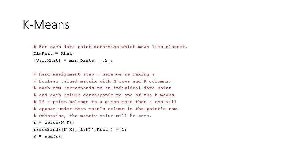
K-Means % For each data point determine which mean lies closest. Old. Khat = Khat; [Val, Khat] = min(Dists, [], 2); % Hard Assignment step - here we're making a % boolean valued matrix with N rows and K columns. % Each row corresponds to an individual data point % and each column corresponds to one of the k-means. % If a point belongs to a given mean then a one will % appear under that mean's column in the point's row. % Otherwise, the matrix value will be zero. r = zeros(N, K); r(sub 2 ind([N K], (1: N)', Khat)) = 1; R = sum(r);

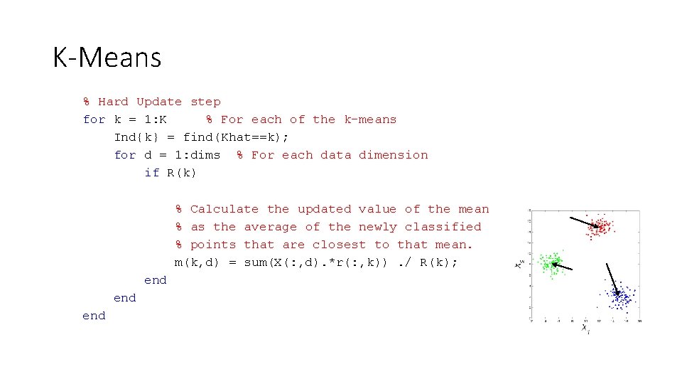
K-Means % Hard Update step for k = 1: K % For each of the k-means Ind{k} = find(Khat==k); for d = 1: dims % For each data dimension if R(k) % Calculate the updated value of the mean % as the average of the newly classified % points that are closest to that mean. m(k, d) = sum(X(: , d). *r(: , k)). / R(k); end end

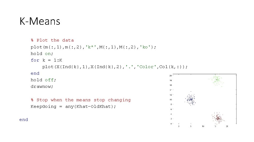
K-Means % Plot the data plot(m(: , 1), m(: , 2), 'k*', M(: , 1), M(: , 2), 'ko'); hold on; for k = 1: K plot(X(Ind{k}, 1), X(Ind{k}, 2), '. ', 'Color', Col(k, : )); end hold off; drawnow; % Stop when the means stop changing Keep. Going = any(Khat-Old. Khat); end

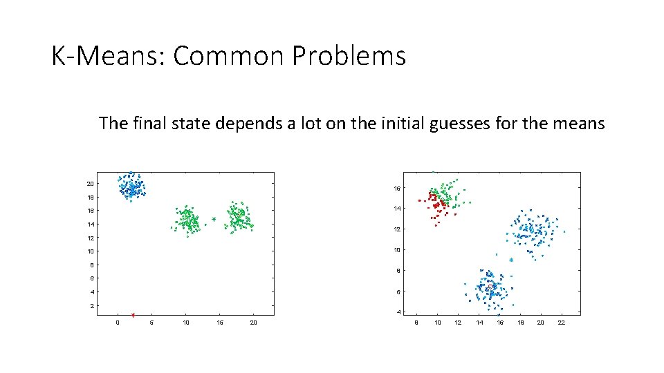
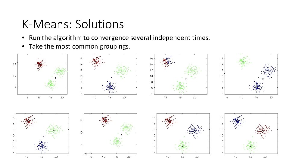
K-Means: Common Problems The final state depends a lot on the initial guesses for the means 20 16 18 14 16 14 12 12 10 10 8 8 6 6 4 2 4 0 5 10 15 20 8 10 12 14 16 18 20 22

K-Means: Solutions • Run the algorithm to convergence several independent times. • Take the most common groupings.

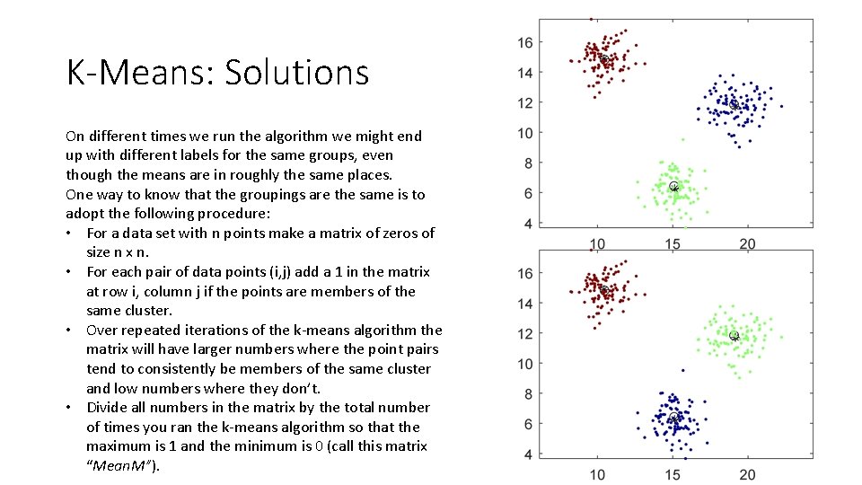
K-Means: Solutions On different times we run the algorithm we might end up with different labels for the same groups, even though the means are in roughly the same places. One way to know that the groupings are the same is to adopt the following procedure: • For a data set with n points make a matrix of zeros of size n x n. • For each pair of data points (i, j) add a 1 in the matrix at row i, column j if the points are members of the same cluster. • Over repeated iterations of the k-means algorithm the matrix will have larger numbers where the point pairs tend to consistently be members of the same cluster and low numbers where they don’t. • Divide all numbers in the matrix by the total number of times you ran the k-means algorithm so that the maximum is 1 and the minimum is 0 (call this matrix “Mean. M”).

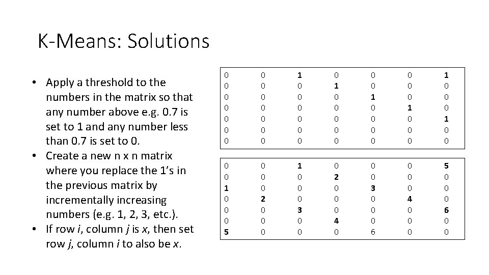
K-Means: Solutions • Apply a threshold to the numbers in the matrix so that any number above e. g. 0. 7 is set to 1 and any number less than 0. 7 is set to 0. • Create a new n x n matrix where you replace the 1’s in the previous matrix by incrementally increasing numbers (e. g. 1, 2, 3, etc. ). • If row i, column j is x, then set row j, column i to also be x. 0 0 0 0 0 0 0 1 0 0 0 0 1 0 0 0 5 0 0 0 2 0 0 0 1 0 0 0 3 0 0 0 2 0 0 0 4 0 0 0 3 0 0 0 6 0 0 0 4 0 0 0 5 0 0 0 6 0 0

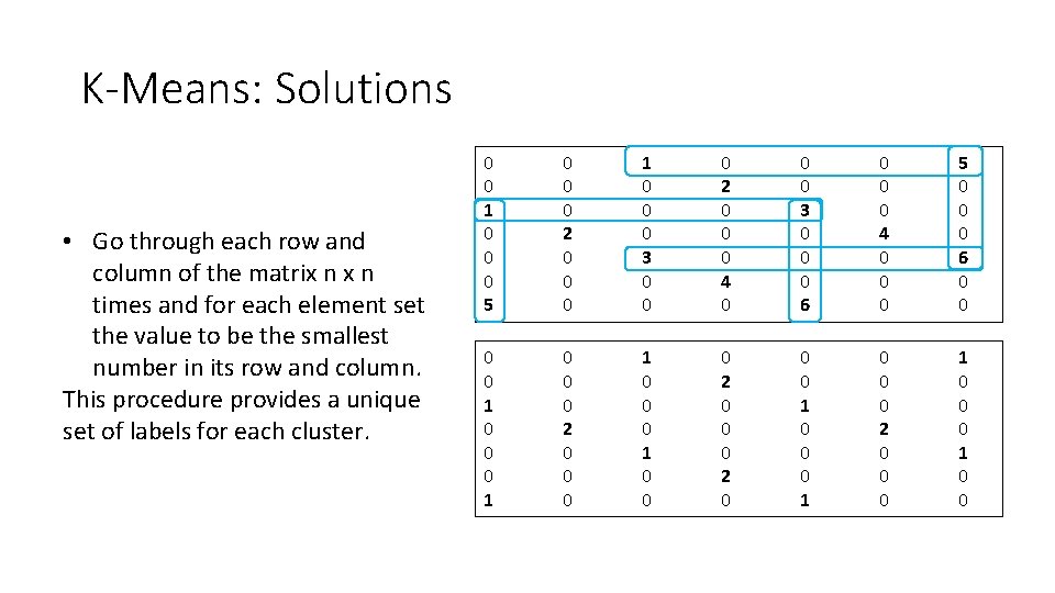
K-Means: Solutions • Go through each row and column of the matrix n times and for each element set the value to be the smallest number in its row and column. This procedure provides a unique set of labels for each cluster. 0 0 1 0 0 0 5 0 0 0 2 0 0 0 1 0 0 0 3 0 0 0 2 0 0 0 4 0 0 0 3 0 0 0 6 0 0 0 4 0 0 0 5 0 0 0 6 0 0 1 0 0 0 2 0 0 0 1 0 0 0 2 0 0 0 1 0 0

K-Means Solutions • Instead of choosing the mean starting locations randomly, you can place them on all possible sets of k data points and apply the procedure just mentioned.

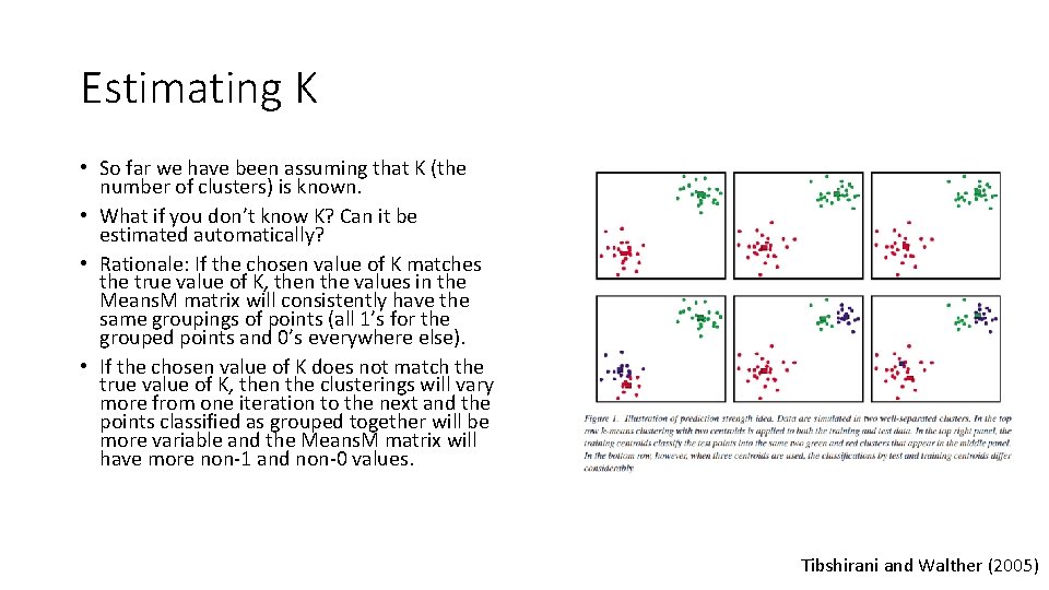
Estimating K • So far we have been assuming that K (the number of clusters) is known. • What if you don’t know K? Can it be estimated automatically? • Rationale: If the chosen value of K matches the true value of K, then the values in the Means. M matrix will consistently have the same groupings of points (all 1’s for the grouped points and 0’s everywhere else). • If the chosen value of K does not match the true value of K, then the clusterings will vary more from one iteration to the next and the points classified as grouped together will be more variable and the Means. M matrix will have more non-1 and non-0 values. Tibshirani and Walther (2005)

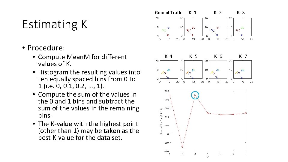
Ground Truth K=1 K=2 K=4 K=5 K=6 K=3 Estimating K • Procedure: • Compute Mean. M for different values of K. • Histogram the resulting values into ten equally spaced bins from 0 to 1 (i. e. 0, 0. 1, 0. 2, …, 1). • Compute the sum of the values in the 0 and 1 bins and subtract the sum of the values in the remaining bins. • The K-value with the highest point (other than 1) may be taken as the best K-value for the data set. K=7

Homework • Try implementing the “Soft K-Means” algorithm presented in the book (Algorithm 20. 7, p. 289) and run it on some toy data (as in our example). • Try running the K-means algorithm on the data in Clustering_2_3 Data. mat. This is a data set of 1600 hand-drawn numbers 2’s and 3’s that are each 16 x 16 pixels in size (256 pixels total). Run the algorithm with 2 clusters and see what you get out. • Hint: to view one image use: imagesc(reshape(X(1, : ), [16 16])');