Clustering Kmeans Clustering Goal Given data Choose classes

Clustering •

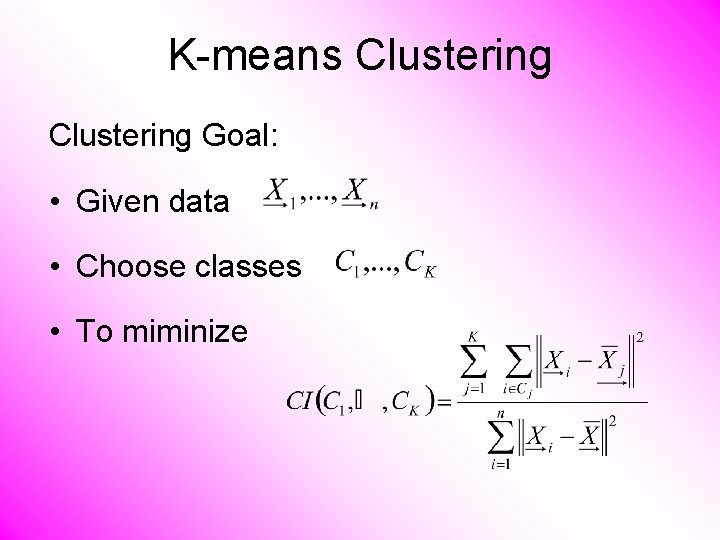
K-means Clustering Goal: • Given data • Choose classes • To miminize

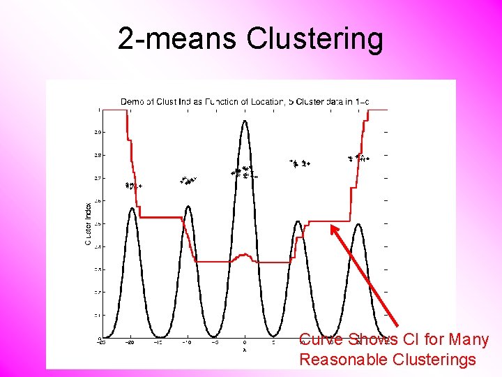
2 -means Clustering Study CI, using simple 1 -d examples • Varying Standard Deviation • Varying Mean • Varying Proportion

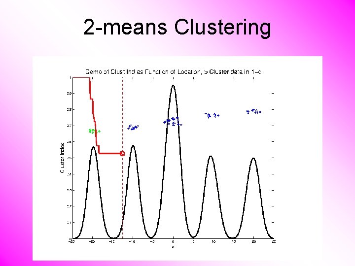
2 -means Clustering

2 -means Clustering Curve Shows CI for Many Reasonable Clusterings

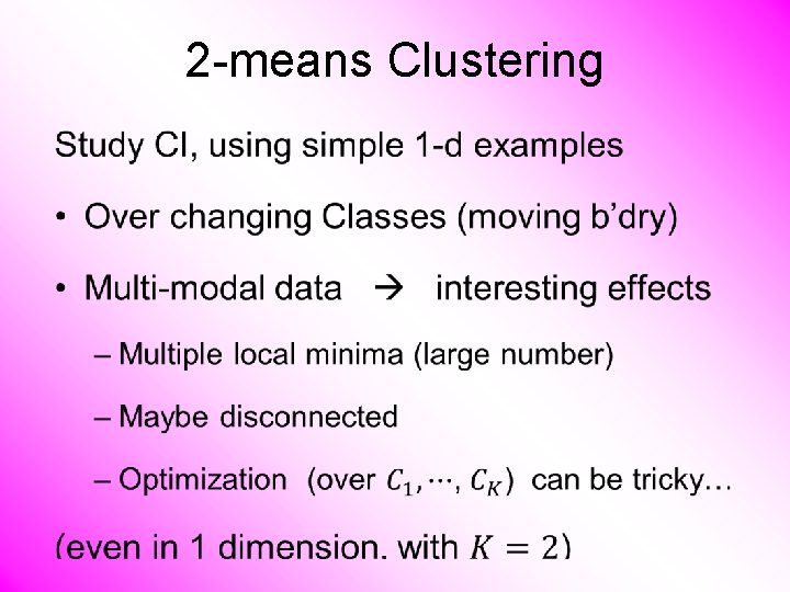
2 -means Clustering •

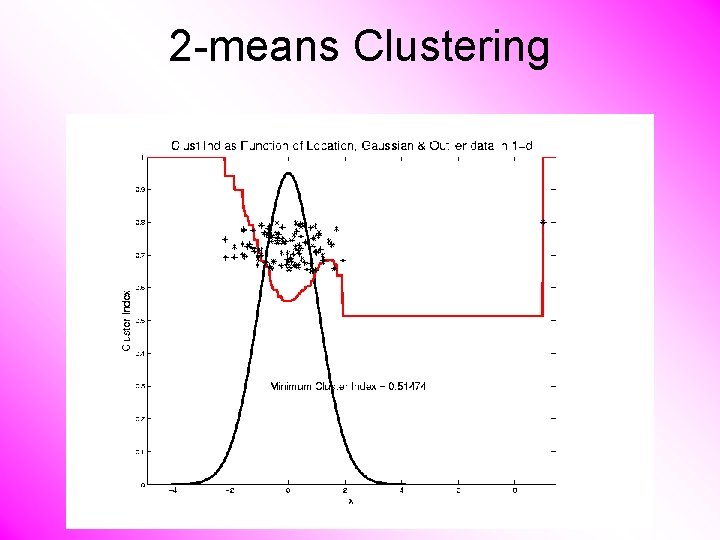
2 -means Clustering Study CI, using simple 1 -d examples • Effect of a single outlier?

2 -means Clustering

SWISS Score Another Application of CI (Cluster Index) Cabanski et al (2010) Idea: Use CI in bioinformatics to “measure quality of data preprocessing” Philosophy: Clusters Are Scientific Goal So Want to Accentuate Them

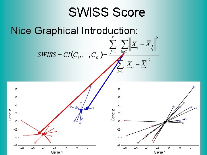
SWISS Score Nice Graphical Introduction:

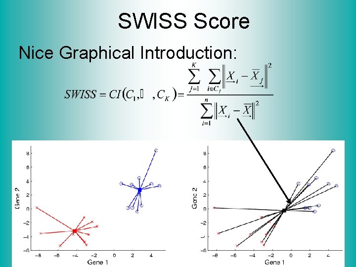
SWISS Score Nice Graphical Introduction:

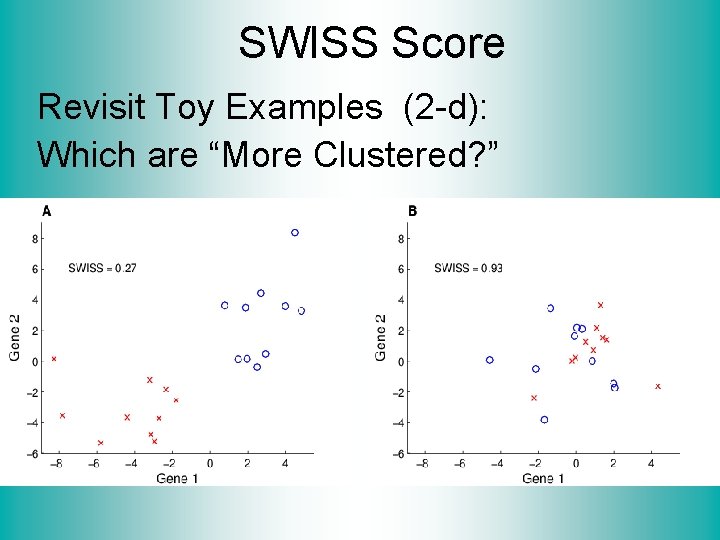
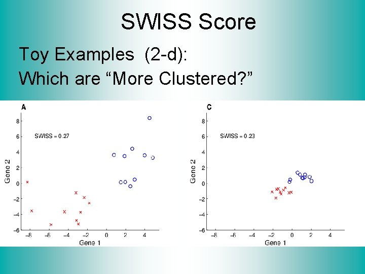
SWISS Score Revisit Toy Examples (2 -d): Which are “More Clustered? ”

SWISS Score Toy Examples (2 -d): Which are “More Clustered? ”

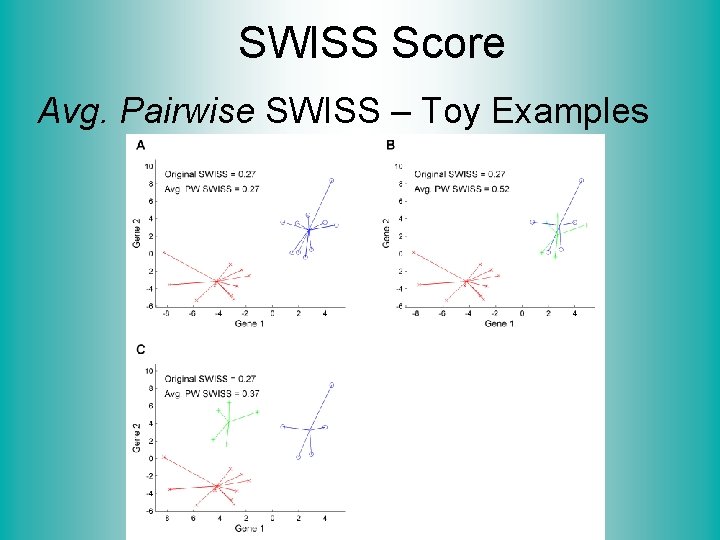
SWISS Score Avg. Pairwise SWISS – Toy Examples

Hiearchical Clustering Idea: Consider Either: Bottom Up Aggregation: One by One Combine Data Top Down Splitting: All Data in One Cluster & Split Through Entire Data Set, to get Dendogram

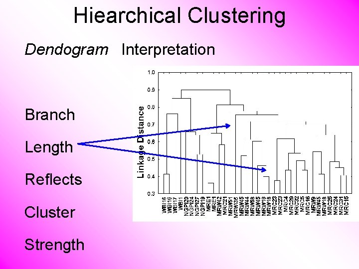
Hiearchical Clustering Dendogram Interpretation Branch Length Reflects Cluster Strength

Sig. Clust • Statistical Significance of Clusters • in HDLSS Data • When is a cluster “really there”? Liu et al (2007), Huang et al (2014)

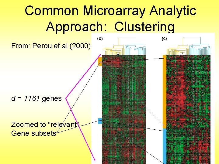
Common Microarray Analytic Approach: Clustering From: Perou et al (2000) d = 1161 genes Zoomed to “relevant” Gene subsets

Interesting Statistical Problem For HDLSS data: n When clusters seem to appear n E. g. found by clustering method n How do we know they are really there? n Question asked by Neil Hayes n Define appropriate statistical significance? n Can we calculate it?

First Approaches: Hypo Testing e. g. Direction, Projection, Permutation Hypothesis test of: Significant difference between sub-populations

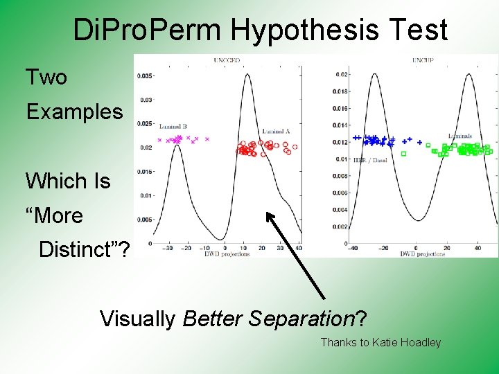
Di. Pro. Perm Hypothesis Test Two Examples Which Is “More Distinct”? Visually Better Separation? Thanks to Katie Hoadley

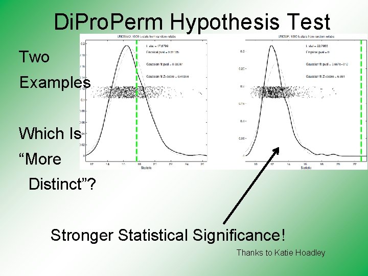
Di. Pro. Perm Hypothesis Test Two Examples Which Is “More Distinct”? Stronger Statistical Significance! Thanks to Katie Hoadley

First Approaches: Hypo Testing e. g. Direction, Projection, Permutation Hypothesis test of: Significant difference between sub-populations n Effective and Accurate n I. e. Sensitive and Specific n There exist several such tests n But critical point is: What result implies about clusters

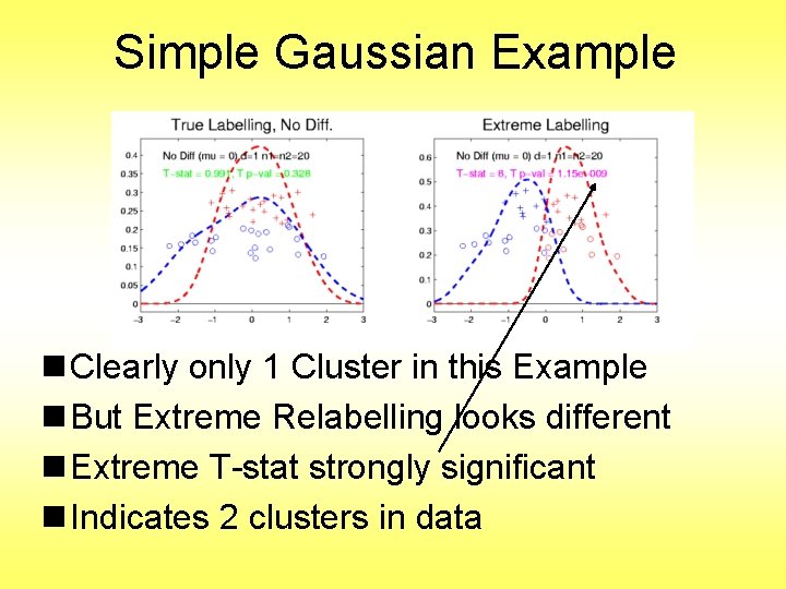
Clarifying Simple Example Why Population Difference Tests cannot indicate clustering n. Andrew Nobel Observation n. For Gaussian Data (Clearly 1 Cluster!) n. Assign Extreme Labels (e. g. by clustering) n. Subpopulations are signif’ly different

Simple Gaussian Example n Clearly only 1 Cluster in this Example n But Extreme Relabelling looks different n Extreme T-stat strongly significant n Indicates 2 clusters in data

Simple Gaussian Example Results: n Random relabelling T-stat is not significant n But extreme T-stat is strongly significant n This comes from clustering operation n Conclude sub-populations are different n Now see that: Not the same as clusters really there n Need a new approach to study clusters

Statistical Significance of Clusters Basis of Sig. Clust Approach: n What defines: A Single Cluster? n A Gaussian distribution (Sarle & Kou 1993) n So define Sig. Clust test based on: n 2 -means cluster index (measure) as statistic n Gaussian null distribution n Currently compute by simulation n Possible to do this analytically? ? ?

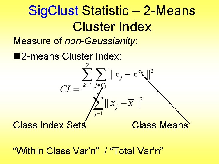
Sig. Clust Statistic – 2 -Means Cluster Index Measure of non-Gaussianity: n 2 -means Cluster Index n Familiar Criterion from k-means Clustering n Within Class Sum of Squared Distances to Class Means n Prefer to divide (normalize) by Overall Sum of Squared Distances to Mean n Puts on scale of proportions

Sig. Clust Statistic – 2 -Means Cluster Index Measure of non-Gaussianity: n 2 -means Cluster Index: Class Index Sets Class Means “Within Class Var’n” / “Total Var’n”

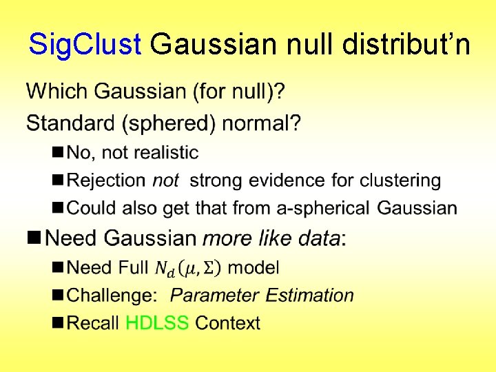
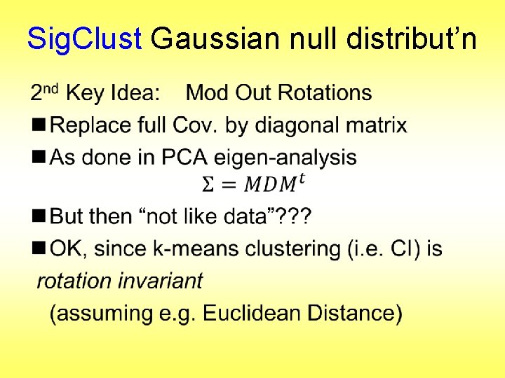
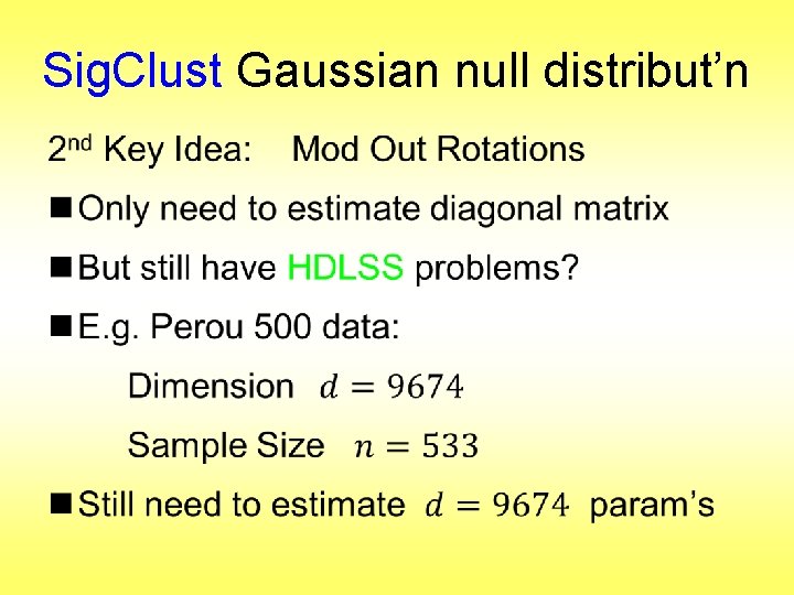
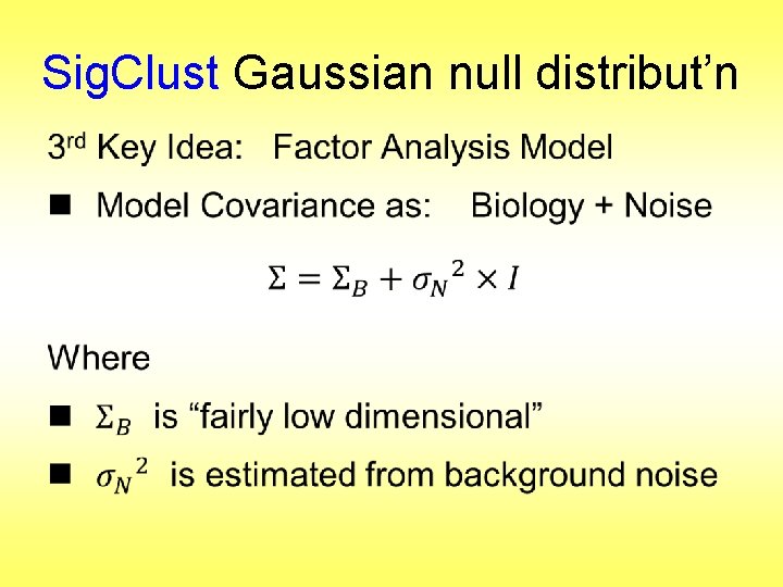
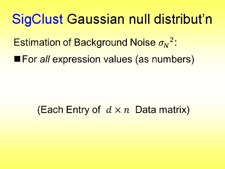
Sig. Clust Gaussian null distribut’n •

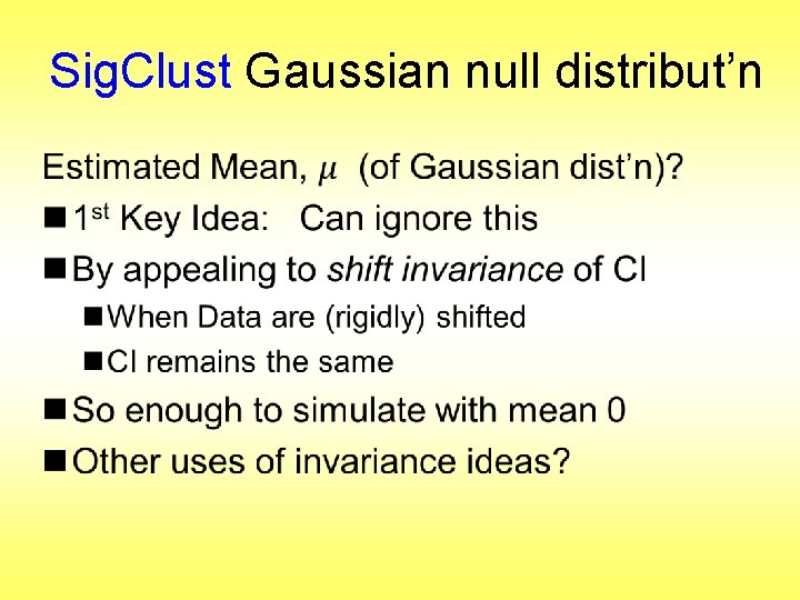
Sig. Clust Gaussian null distribut’n •

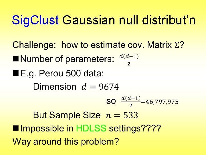
Sig. Clust Gaussian null distribut’n •

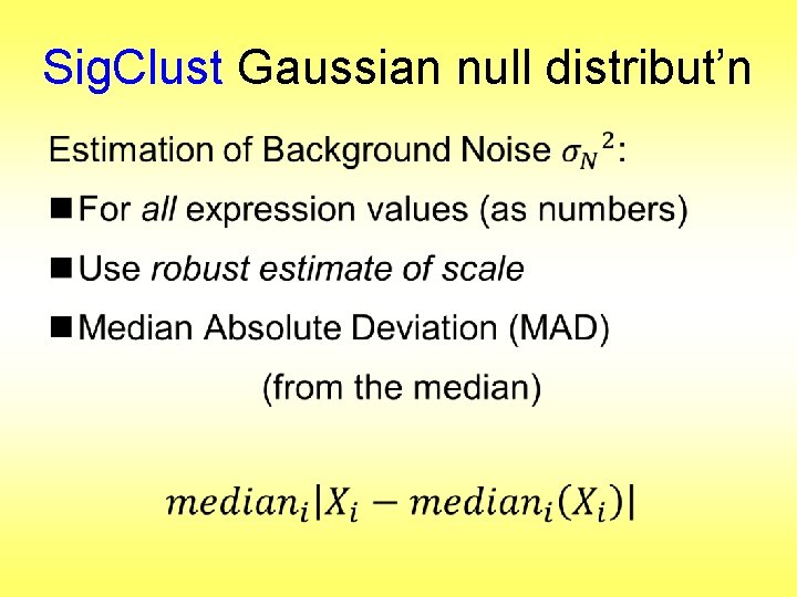
Sig. Clust Gaussian null distribut’n •

Sig. Clust Gaussian null distribut’n •

Sig. Clust Gaussian null distribut’n •

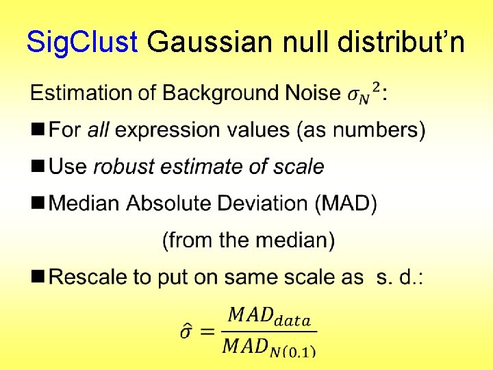
Sig. Clust Gaussian null distribut’n •

Sig. Clust Gaussian null distribut’n •

Sig. Clust Gaussian null distribut’n •

Sig. Clust Gaussian null distribut’n •

Sig. Clust Gaussian null distribut’n •

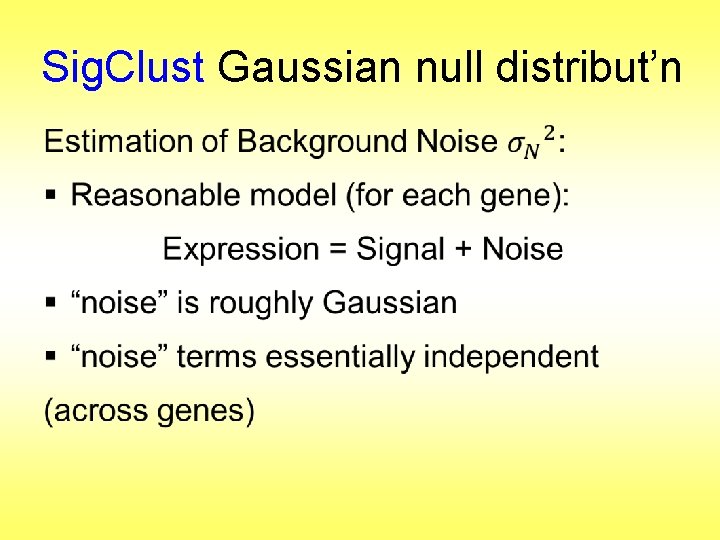
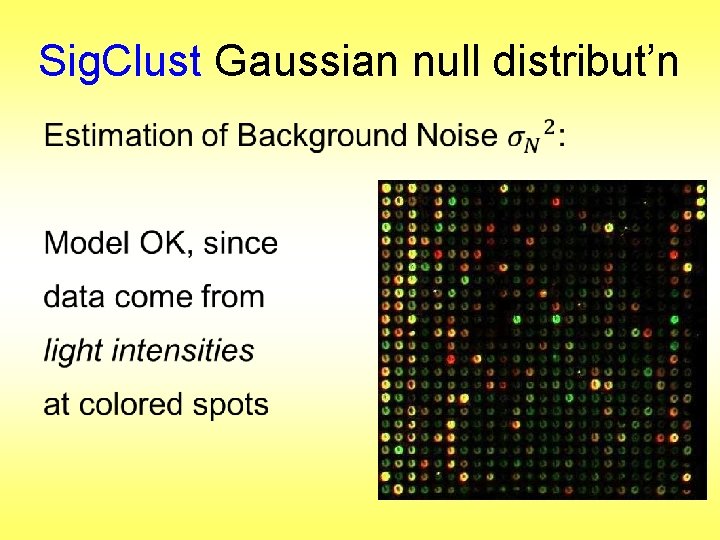
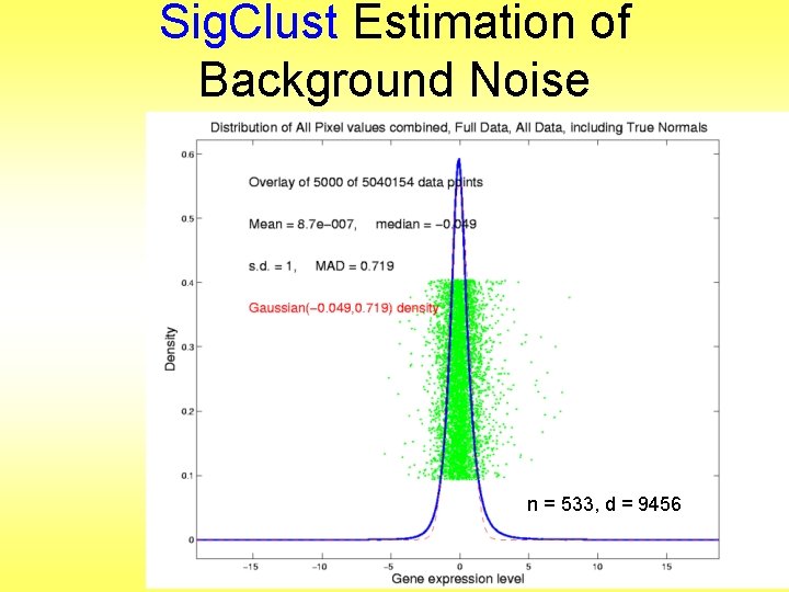
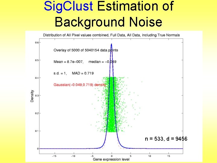
Sig. Clust Estimation of Background Noise n = 533, d = 9456

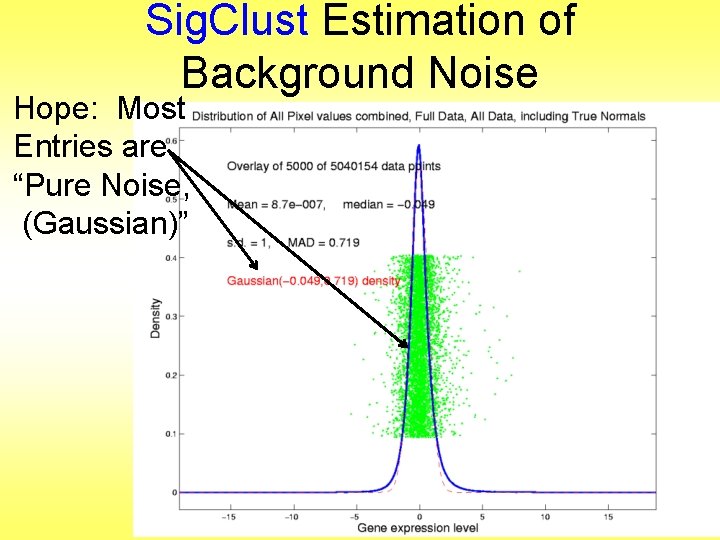
Sig. Clust Estimation of Background Noise Hope: Most Entries are “Pure Noise, (Gaussian)”

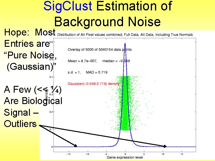
Sig. Clust Estimation of Background Noise Hope: Most Entries are “Pure Noise, (Gaussian)” A Few (<< ¼) Are Biological Signal – Outliers

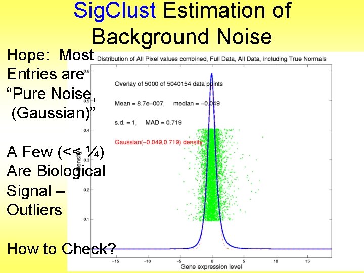
Sig. Clust Estimation of Background Noise Hope: Most Entries are “Pure Noise, (Gaussian)” A Few (<< ¼) Are Biological Signal – Outliers How to Check?

Q-Q plots An aside: Fitting probability distributions to data • Does Gaussian distribution “fit”? ? ? • If not, why not? • Fit in some part of the distribution? (e. g. in the middle only? )

Q-Q plots Approaches to: Fitting probability distributions to data • Histograms • Kernel Density Estimates Drawbacks: often not best view (for determining goodness of fit)

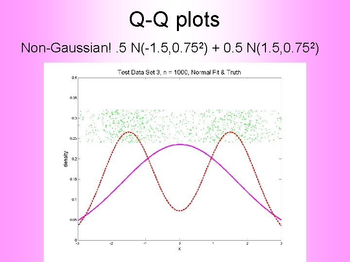
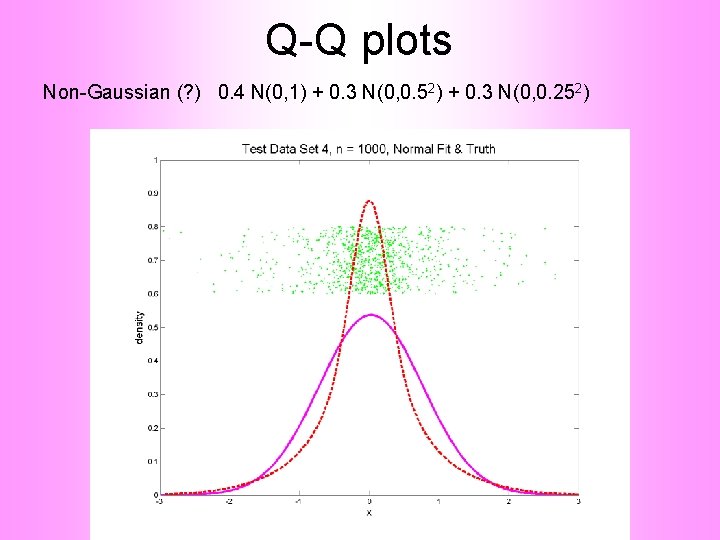
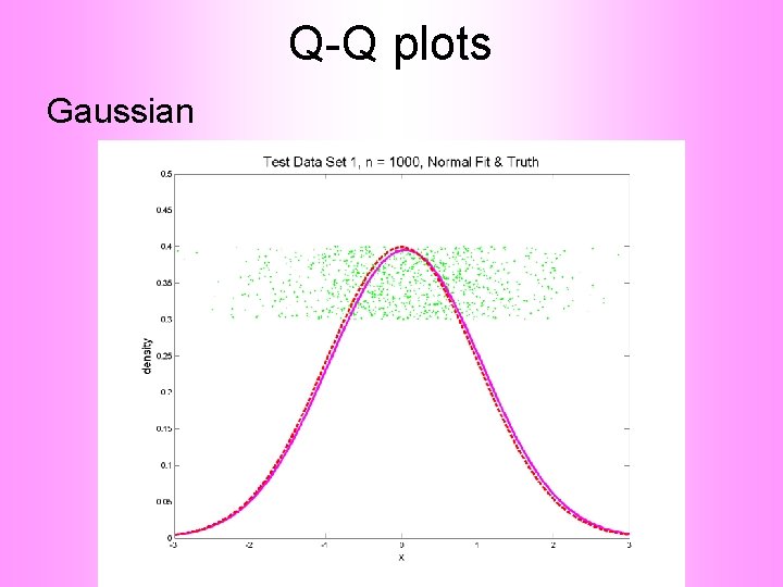
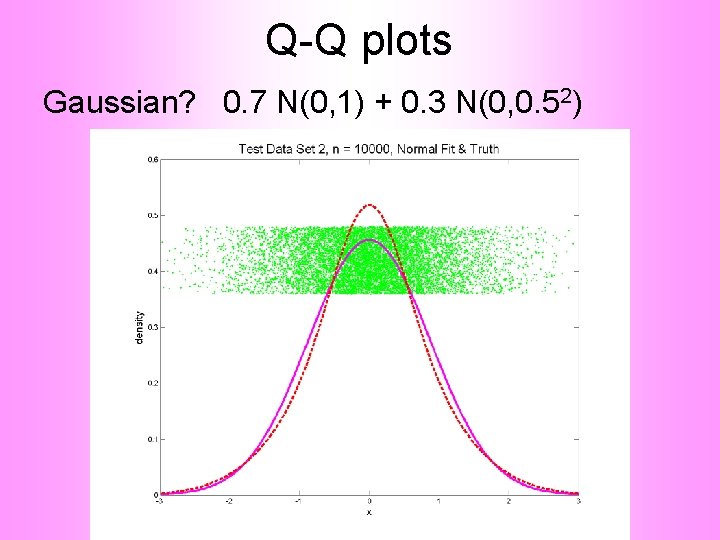
Q-Q plots Consider Testbed of 4 Toy Examples: Ø non-Gaussian! Ø non-Gaussian(? ) Ø Gaussian? (Will use these names several times)

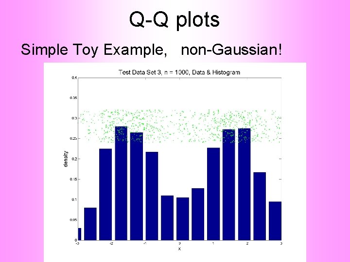
Q-Q plots Simple Toy Example, non-Gaussian!

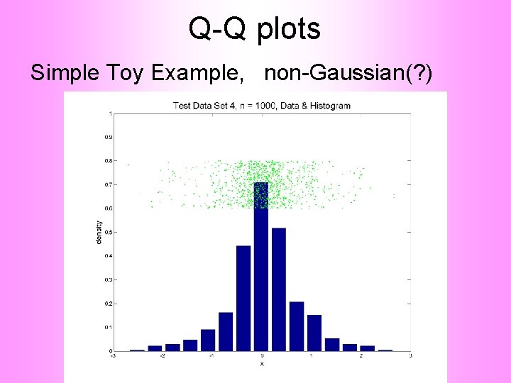
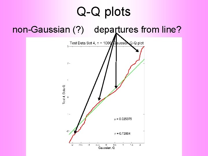
Q-Q plots Simple Toy Example, non-Gaussian(? )

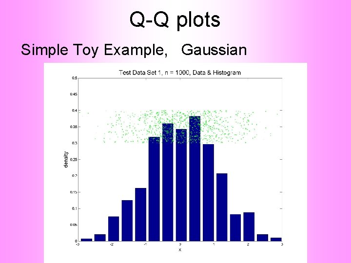
Q-Q plots Simple Toy Example, Gaussian

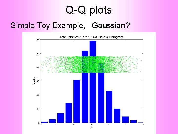
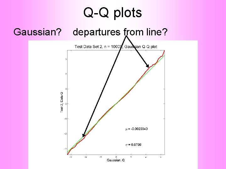
Q-Q plots Simple Toy Example, Gaussian?

Q-Q plots Notes: • Bimodal see non-Gaussian with histo • Other cases: hard to see • Conclude: Histogram poor at assessing Gauss’ity

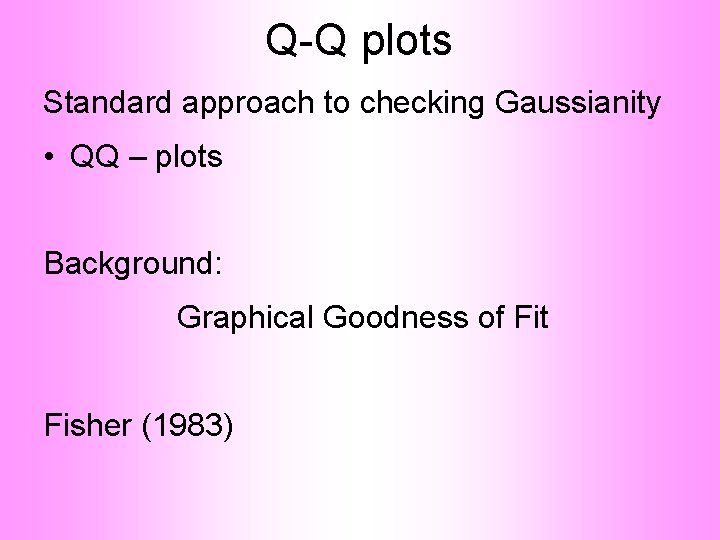
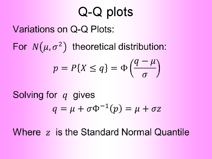
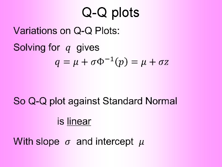
Q-Q plots Standard approach to checking Gaussianity • QQ – plots Background: Graphical Goodness of Fit Fisher (1983)

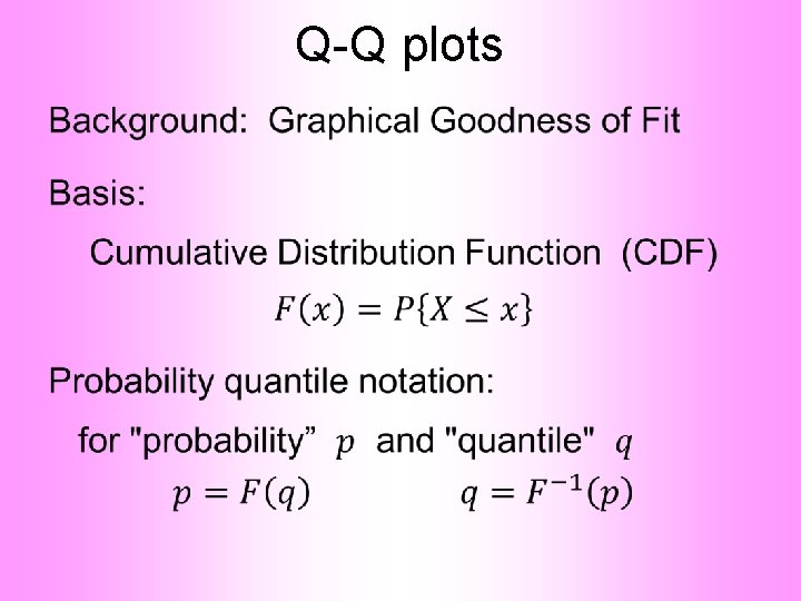
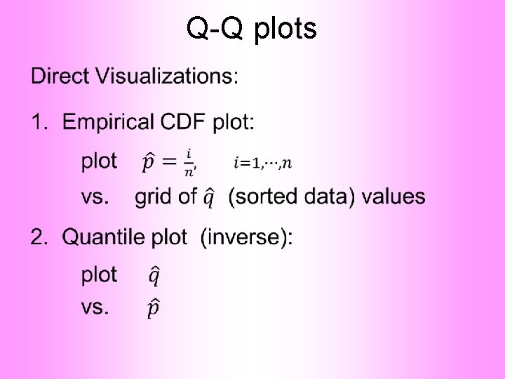
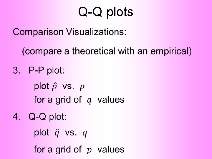
Q-Q plots •

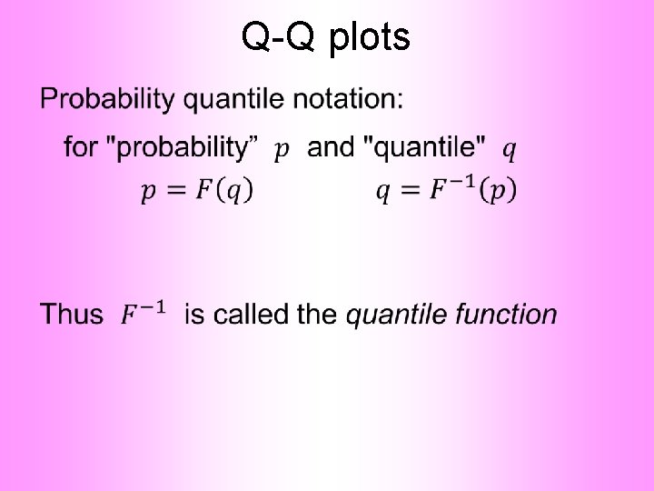
Q-Q plots •

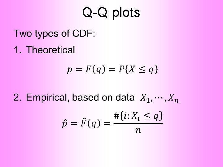
Q-Q plots •

Q-Q plots •

Q-Q plots •

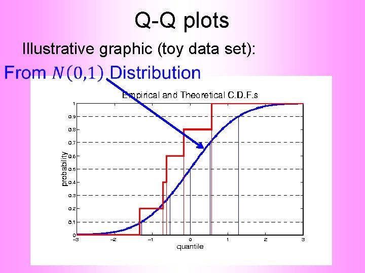
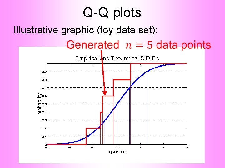
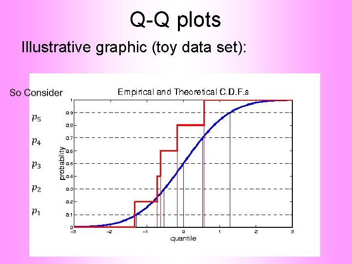
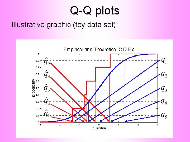
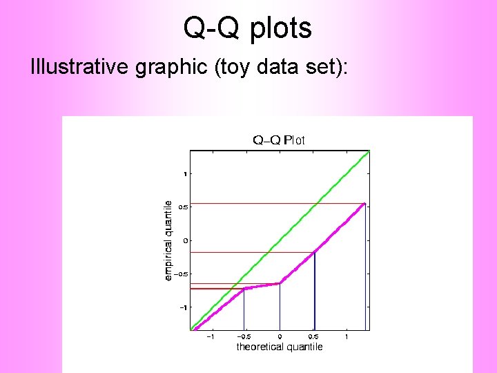
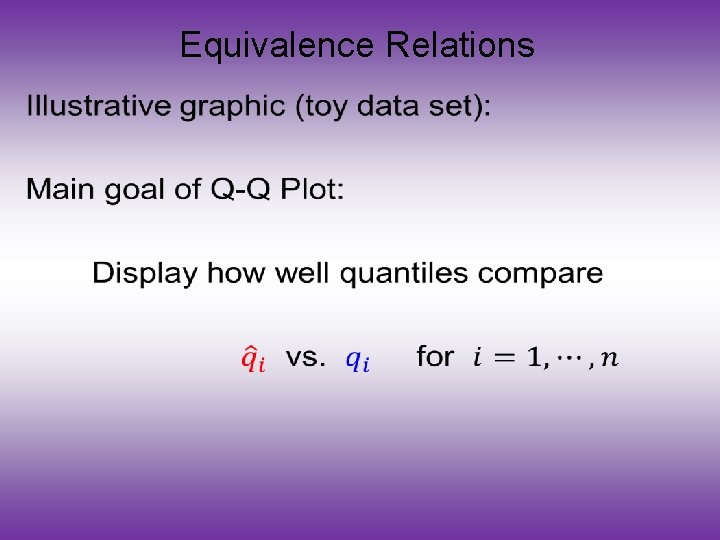
Q-Q plots Illustrative graphic (toy data set):

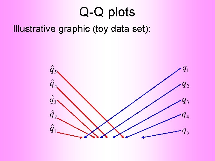
Q-Q plots Illustrative graphic (toy data set):

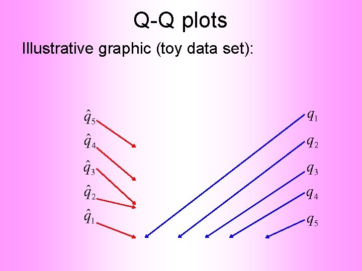
Q-Q plots Illustrative graphic (toy data set):

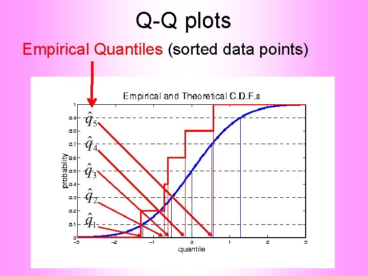
Q-Q plots Empirical Quantiles (sorted data points)

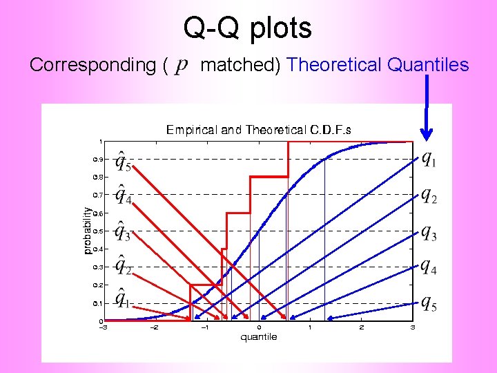
Q-Q plots Corresponding ( matched) Theoretical Quantiles

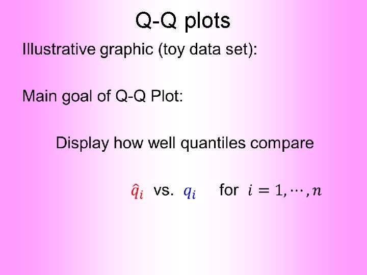
Q-Q plots •

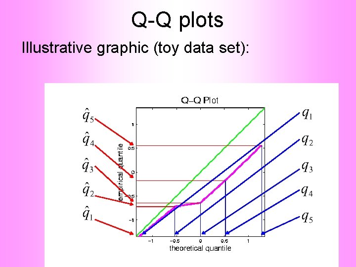
Q-Q plots Illustrative graphic (toy data set):

Q-Q plots Illustrative graphic (toy data set):

Q-Q plots Illustrative graphic (toy data set):

Q-Q plots Illustrative graphic (toy data set):

Q-Q plots Illustrative graphic (toy data set):

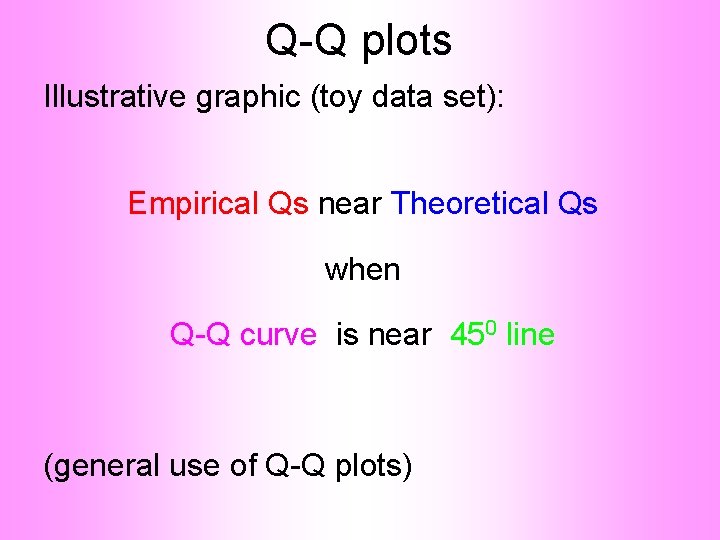
Q-Q plots Illustrative graphic (toy data set): Empirical Qs near Theoretical Qs when Q-Q curve is near 450 line (general use of Q-Q plots)

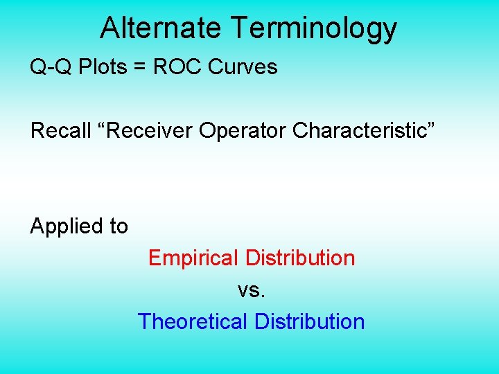
Alternate Terminology Q-Q Plots = ROC Curves Recall “Receiver Operator Characteristic” Applied to Empirical Distribution vs. Theoretical Distribution

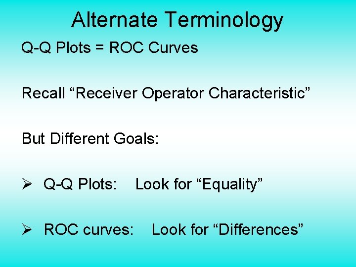
Alternate Terminology Q-Q Plots = ROC Curves Recall “Receiver Operator Characteristic” But Different Goals: Ø Q-Q Plots: Look for “Equality” Ø ROC curves: Look for “Differences”

Alternate Terminology Q-Q Plots = ROC Curves P-P Plot = Curve that Highlights Different Distributional Aspects Statistical Folklore: Q-Q Highlights Tails, So Usually More Useful

Alternate Terminology Q-Q Plots = ROC Curves Related Measures: Precision & Recall

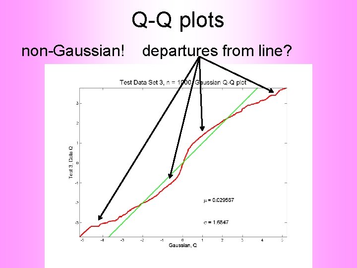
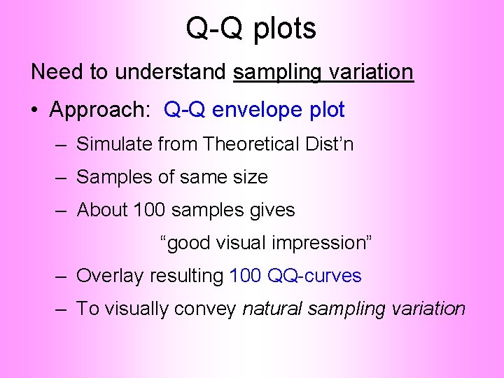
Q-Q plots non-Gaussian! departures from line?

Q-Q plots non-Gaussian! departures from line? • Seems different from line? • 2 modes turn into wiggles? • Less strong feature • Been proposed to study modality

Q-Q plots non-Gaussian (? ) departures from line?

Q-Q plots non-Gaussian (? ) departures from line? • Seems different from line? • Harder to say this time? • What is signal & what is noise? • Need to understand sampling variation

Q-Q plots Gaussian? departures from line?

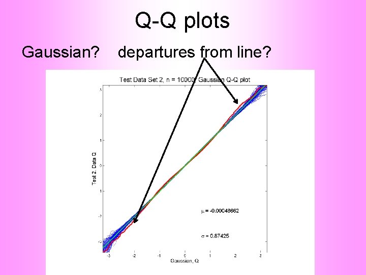
Q-Q plots Gaussian? departures from line? • Looks much like? • Wiggles all random variation? • But there are n = 10, 000 data points… • How to assess signal & noise? • Need to understand sampling variation

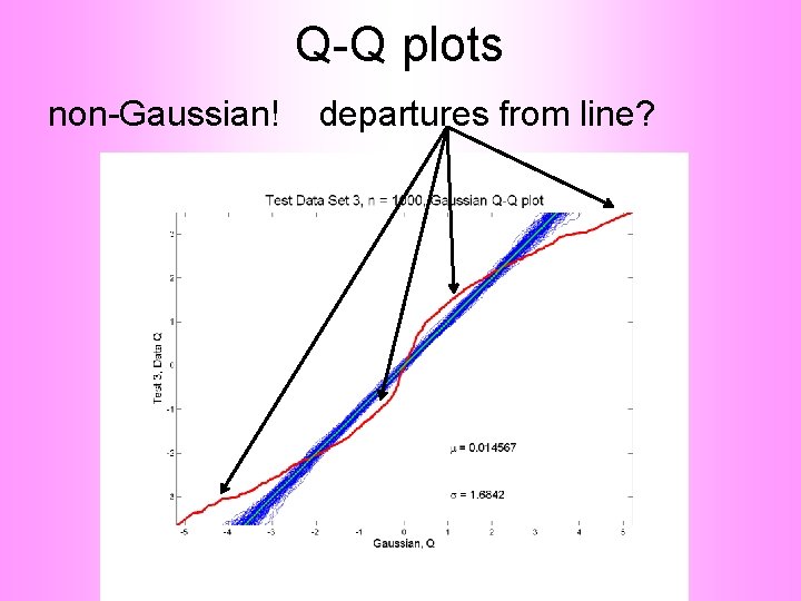
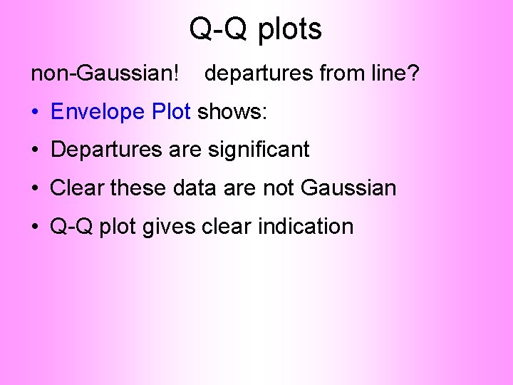
Q-Q plots Need to understand sampling variation • Approach: Q-Q envelope plot – Simulate from Theoretical Dist’n – Samples of same size – About 100 samples gives “good visual impression” – Overlay resulting 100 QQ-curves – To visually convey natural sampling variation

Q-Q plots non-Gaussian! departures from line?

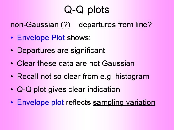
Q-Q plots non-Gaussian! departures from line? • Envelope Plot shows: • Departures are significant • Clear these data are not Gaussian • Q-Q plot gives clear indication

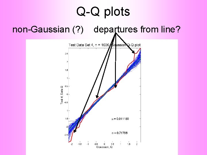
Q-Q plots non-Gaussian (? ) departures from line?

Q-Q plots non-Gaussian (? ) departures from line? • Envelope Plot shows: • Departures are significant • Clear these data are not Gaussian • Recall not so clear from e. g. histogram • Q-Q plot gives clear indication • Envelope plot reflects sampling variation

Q-Q plots Gaussian? departures from line?

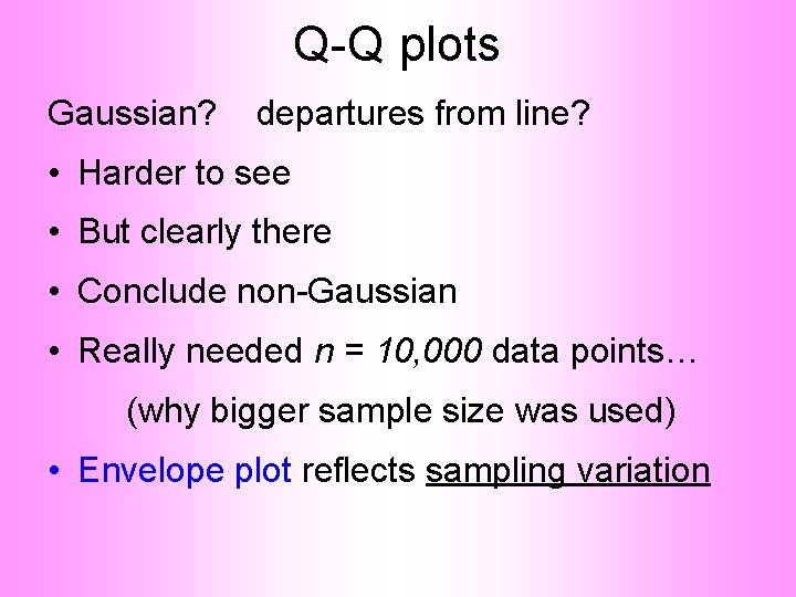
Q-Q plots Gaussian? departures from line? • Harder to see • But clearly there • Conclude non-Gaussian • Really needed n = 10, 000 data points… (why bigger sample size was used) • Envelope plot reflects sampling variation

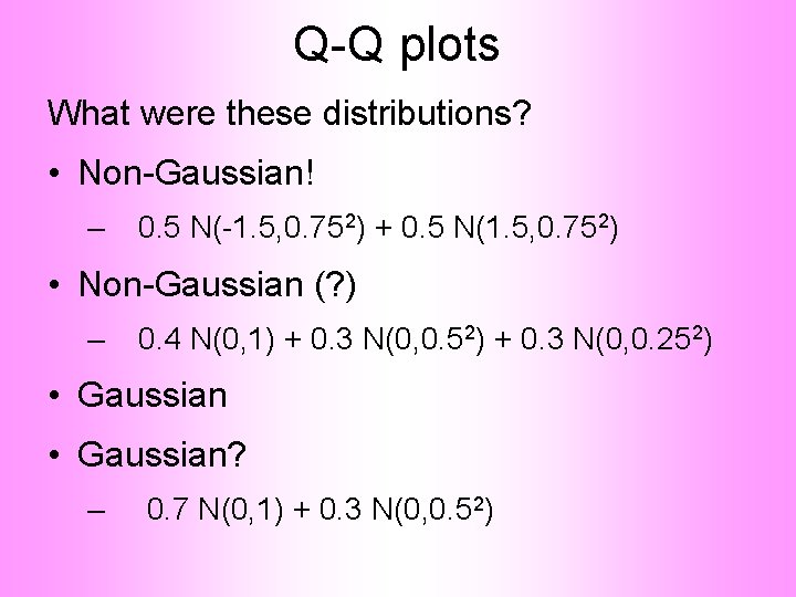
Q-Q plots What were these distributions? • Non-Gaussian! – 0. 5 N(-1. 5, 0. 752) + 0. 5 N(1. 5, 0. 752) • Non-Gaussian (? ) – 0. 4 N(0, 1) + 0. 3 N(0, 0. 52) + 0. 3 N(0, 0. 252) • Gaussian? – 0. 7 N(0, 1) + 0. 3 N(0, 0. 52)

Q-Q plots Non-Gaussian!. 5 N(-1. 5, 0. 752) + 0. 5 N(1. 5, 0. 752)

Q-Q plots Non-Gaussian (? ) 0. 4 N(0, 1) + 0. 3 N(0, 0. 52) + 0. 3 N(0, 0. 252)

Q-Q plots Gaussian

Q-Q plots Gaussian? 0. 7 N(0, 1) + 0. 3 N(0, 0. 52)

Q-Q plots •

Q-Q plots •

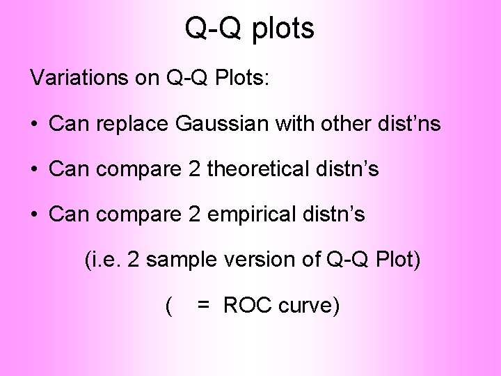
Q-Q plots Variations on Q-Q Plots: • Can replace Gaussian with other dist’ns • Can compare 2 theoretical distn’s • Can compare 2 empirical distn’s (i. e. 2 sample version of Q-Q Plot) ( = ROC curve)

Sig. Clust Estimation of Background Noise n = 533, d = 9456

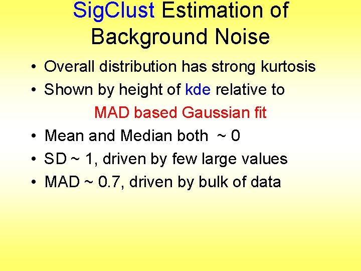
Sig. Clust Estimation of Background Noise • Overall distribution has strong kurtosis • Shown by height of kde relative to MAD based Gaussian fit • Mean and Median both ~ 0 • SD ~ 1, driven by few large values • MAD ~ 0. 7, driven by bulk of data

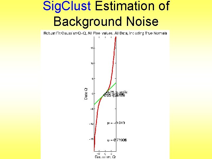
Sig. Clust Estimation of Background Noise • Central part of distribution “seems to look Gaussian” • But recall density does not provide great diagnosis of Gaussianity • Better to look at Q-Q plot

Sig. Clust Estimation of Background Noise

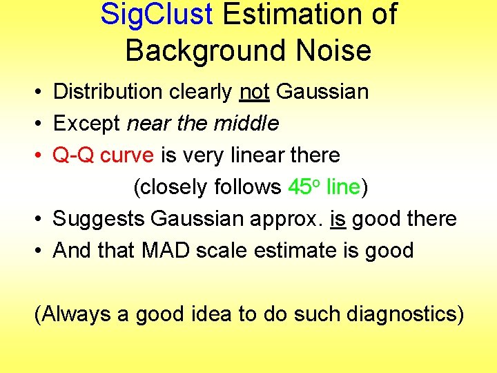
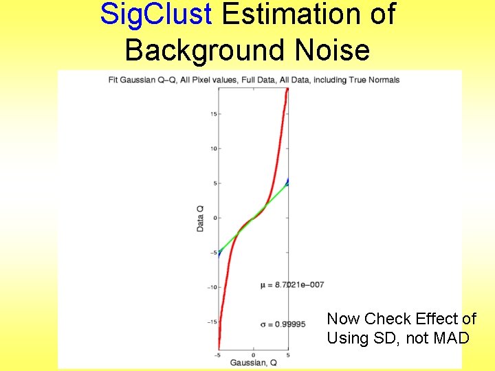
Sig. Clust Estimation of Background Noise • Distribution clearly not Gaussian • Except near the middle • Q-Q curve is very linear there (closely follows 45 o line) • Suggests Gaussian approx. is good there • And that MAD scale estimate is good (Always a good idea to do such diagnostics)

Sig. Clust Estimation of Background Noise Now Check Effect of Using SD, not MAD

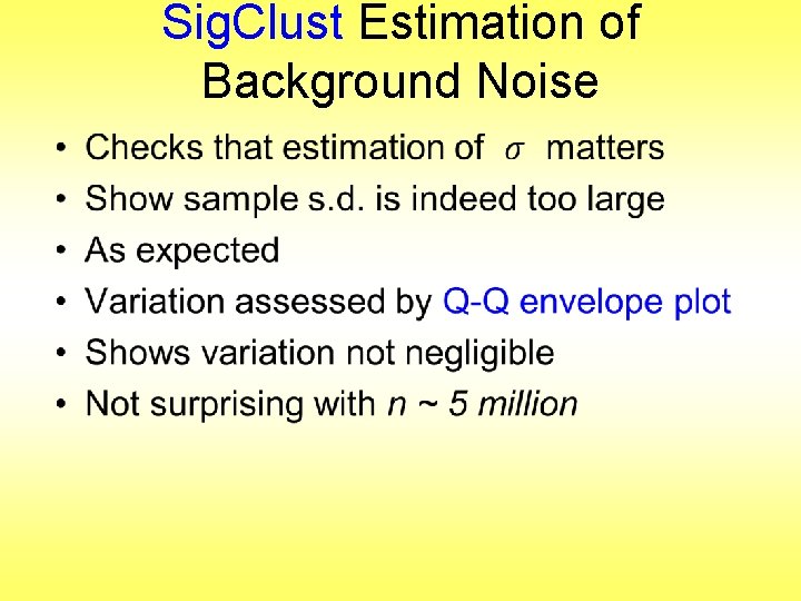
Sig. Clust Estimation of Background Noise •

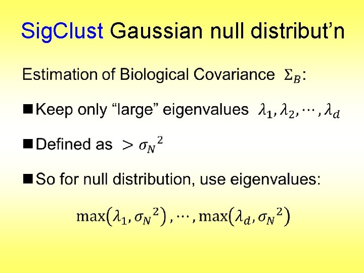
Sig. Clust Gaussian null distribut’n •

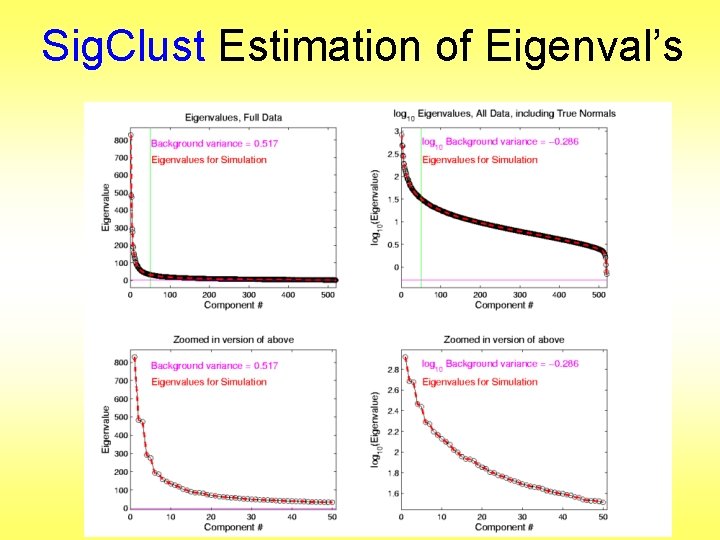
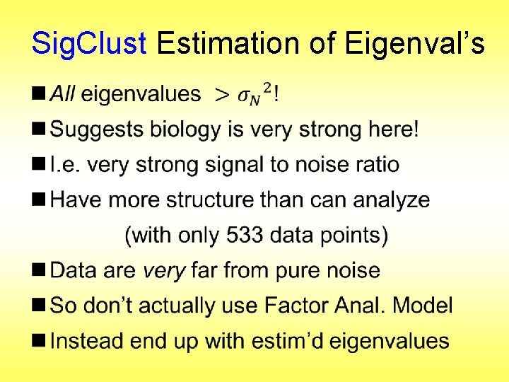
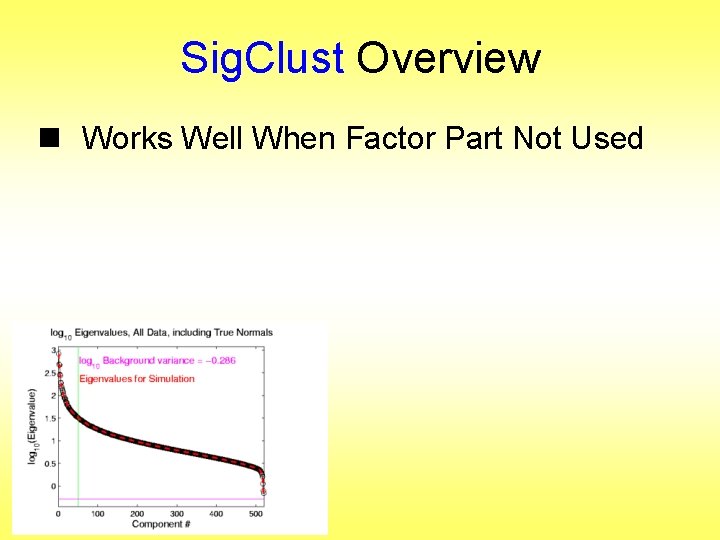
Sig. Clust Estimation of Eigenval’s

Sig. Clust Estimation of Eigenval’s •

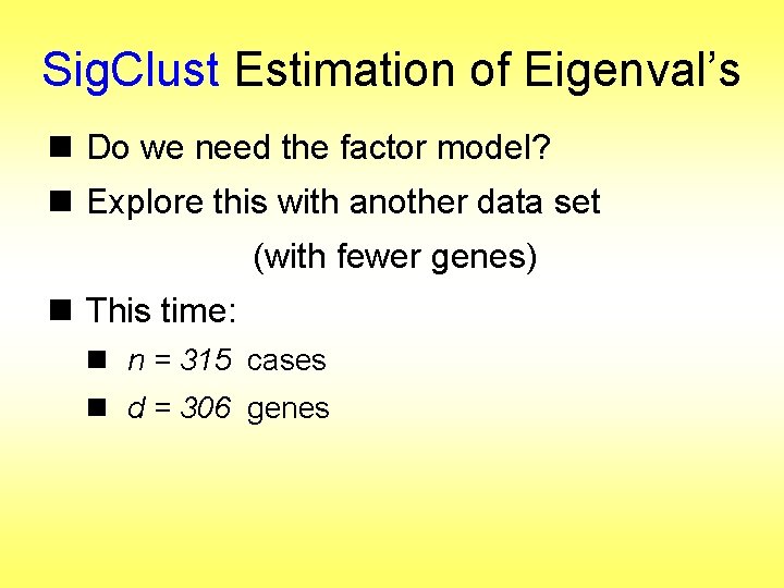
Sig. Clust Estimation of Eigenval’s n Do we need the factor model? n Explore this with another data set (with fewer genes) n This time: n n = 315 cases n d = 306 genes

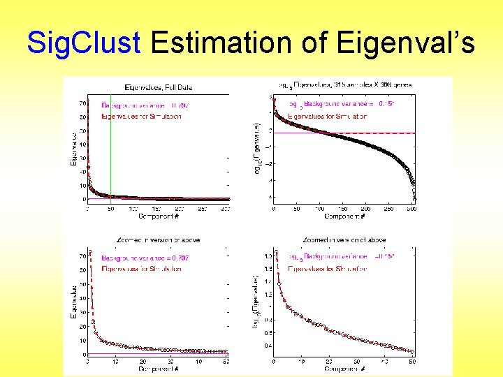
Sig. Clust Estimation of Eigenval’s

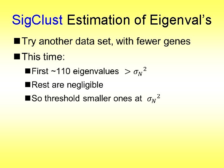
Sig. Clust Estimation of Eigenval’s •

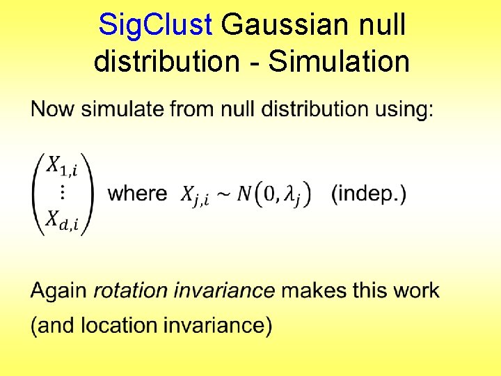
Sig. Clust Gaussian null distribution - Simulation •

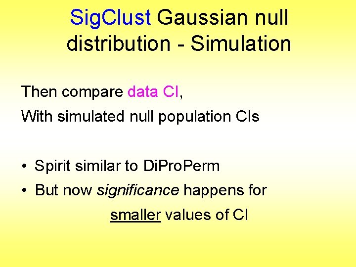
Sig. Clust Gaussian null distribution - Simulation Then compare data CI, With simulated null population CIs • Spirit similar to Di. Pro. Perm • But now significance happens for smaller values of CI

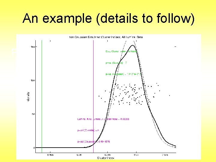
An example (details to follow) P-val = 0. 0045

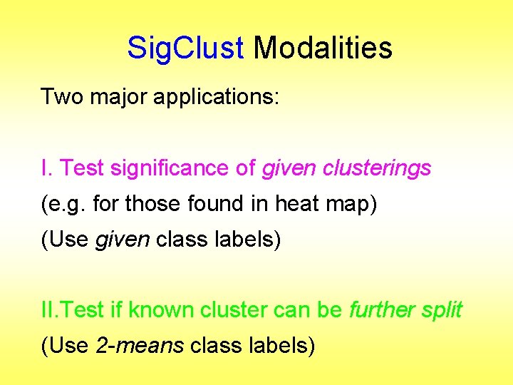
Sig. Clust Modalities Two major applications: I. Test significance of given clusterings (e. g. for those found in heat map) (Use given class labels) II. Test if known cluster can be further split (Use 2 -means class labels)

Sig. Clust Real Data Results Analyze Perou 500 breast cancer data (large cross study combined data set) Current folklore: 5 classes § Luminal A § Luminal B § Normal § Her 2 § Basal

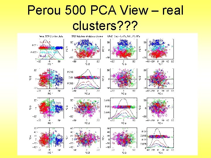
Perou 500 PCA View – real clusters? ? ?

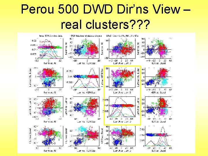
Perou 500 DWD Dir’ns View – real clusters? ? ?

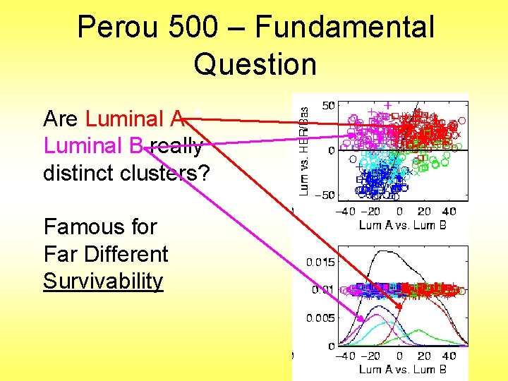
Perou 500 – Fundamental Question Are Luminal A & Luminal B really distinct clusters? Famous for Far Different Survivability

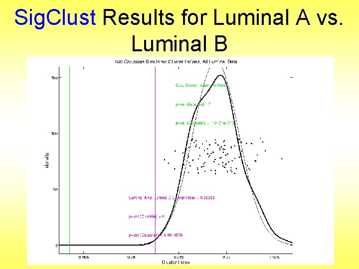
Sig. Clust Results for Luminal A vs. Luminal B P-val = 0. 0045

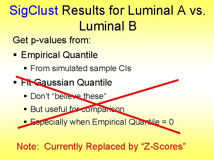
Sig. Clust Results for Luminal A vs. Luminal B Get p-values from: § Empirical Quantile § From simulated sample CIs § Fit Gaussian Quantile § Don’t “believe these” § But useful for comparison § Especially when Empirical Quantile = 0 Note: Currently Replaced by “Z-Scores”

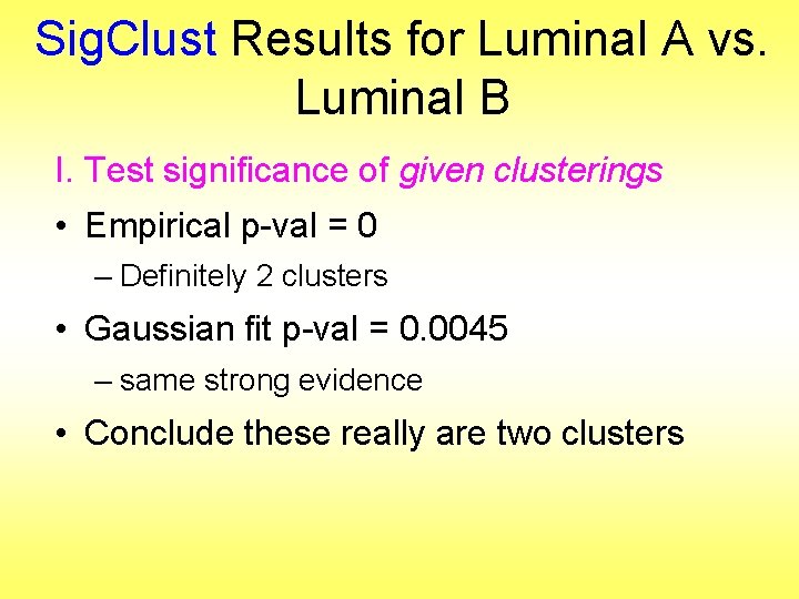
Sig. Clust Results for Luminal A vs. Luminal B I. Test significance of given clusterings • Empirical p-val = 0 – Definitely 2 clusters • Gaussian fit p-val = 0. 0045 – same strong evidence • Conclude these really are two clusters

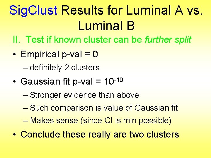
Sig. Clust Results for Luminal A vs. Luminal B II. Test if known cluster can be further split • Empirical p-val = 0 – definitely 2 clusters • Gaussian fit p-val = 10 -10 – Stronger evidence than above – Such comparison is value of Gaussian fit – Makes sense (since CI is min possible) • Conclude these really are two clusters

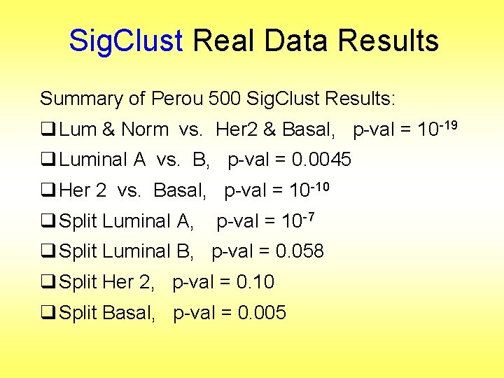
Sig. Clust Real Data Results Summary of Perou 500 Sig. Clust Results: q Lum & Norm vs. Her 2 & Basal, p-val = 10 -19 q Luminal A vs. B, p-val = 0. 0045 q Her 2 vs. Basal, p-val = 10 -10 q Split Luminal A, p-val = 10 -7 q Split Luminal B, p-val = 0. 058 q Split Her 2, p-val = 0. 10 q Split Basal, p-val = 0. 005

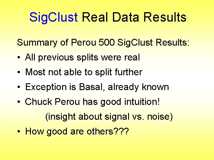
Sig. Clust Real Data Results Summary of Perou 500 Sig. Clust Results: • All previous splits were real • Most not able to split further • Exception is Basal, already known • Chuck Perou has good intuition! (insight about signal vs. noise) • How good are others? ? ?

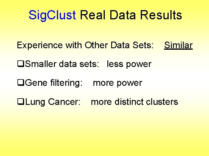
Sig. Clust Real Data Results Experience with Other Data Sets: Similar q. Smaller data sets: less power q. Gene filtering: more power q. Lung Cancer: more distinct clusters

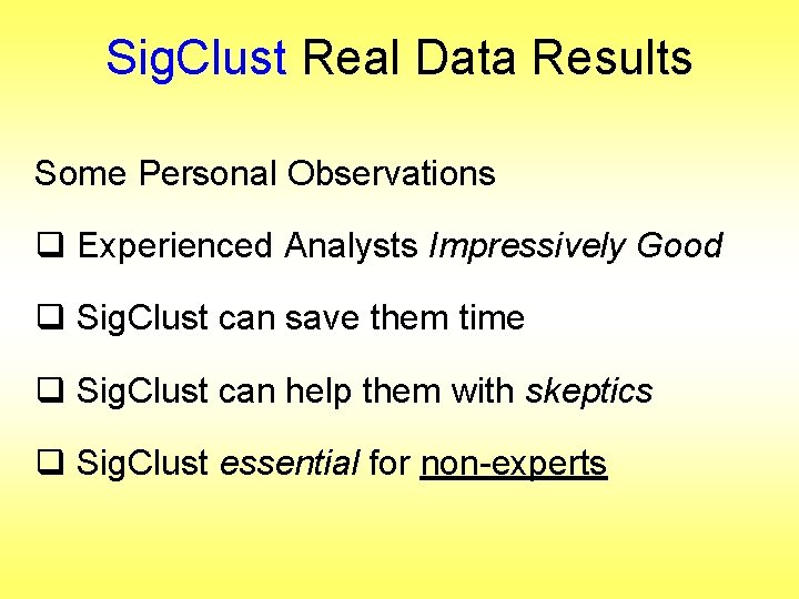
Sig. Clust Real Data Results Some Personal Observations q Experienced Analysts Impressively Good q Sig. Clust can save them time q Sig. Clust can help them with skeptics q Sig. Clust essential for non-experts

Sig. Clust Overview n Works Well When Factor Part Not Used

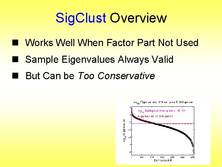
Sig. Clust Overview n Works Well When Factor Part Not Used n Sample Eigenvalues Always Valid n But Can be Too Conservative

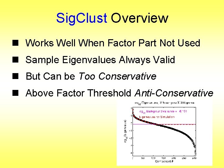
Sig. Clust Overview n Works Well When Factor Part Not Used n Sample Eigenvalues Always Valid n But Can be Too Conservative n Above Factor Threshold Anti-Conservative

Sig. Clust Overview n Works Well When Factor Part Not Used n Sample Eigenvalues Always Valid n But Can be Too Conservative n Above Factor Threshold Anti-Conservative n Problem Fixed by Soft Thresholding (Huang et al, 2014)

Sig. Clust Open Problems n Improved Eigenvalue Estimation (Random Matrix Theory) n More attention to Local Minima in 2 means Clustering n Theoretical Null Distributions n Inference for k > 2 means Clustering n Multiple Comparison Issues

Big Picture •

Shapes As Data Objects Several Different Notions of Shape Oldest and Best Known (in Statistics): Landmark Based

Shapes As Data Objects •

Shapes As Data Objects Landmark Based Shape Analysis: v Kendall (et al 1999) v Bookstein (1991) v Dryden & Mardia (1998, revision coming) Recommended as Most Accessible

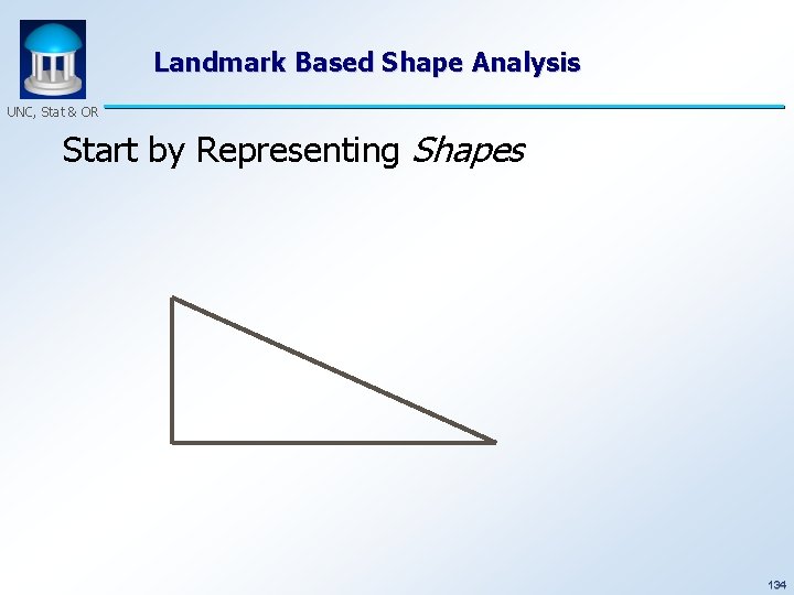
Landmark Based Shape Analysis UNC, Stat & OR Start by Representing Shapes 134

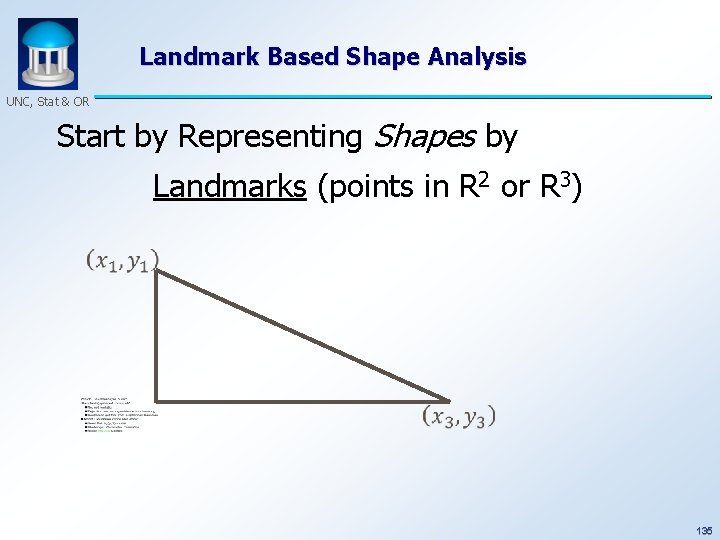
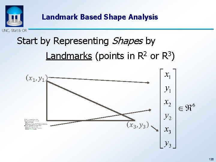
Landmark Based Shape Analysis UNC, Stat & OR Start by Representing Shapes by Landmarks (points in R 2 or R 3) 135

Landmark Based Shape Analysis UNC, Stat & OR Start by Representing Shapes by Landmarks (points in R 2 or R 3) 136

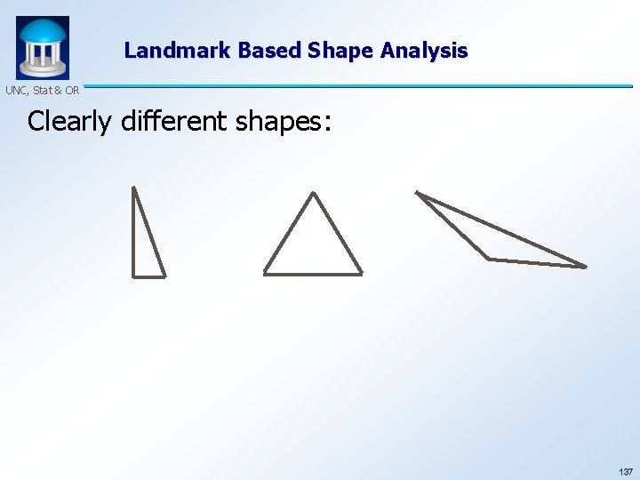
Landmark Based Shape Analysis UNC, Stat & OR Clearly different shapes: 137

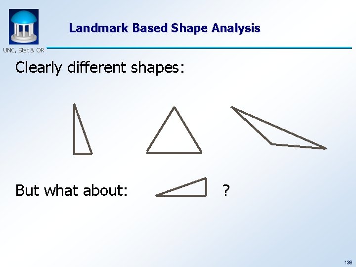
Landmark Based Shape Analysis UNC, Stat & OR Clearly different shapes: But what about: ? 138

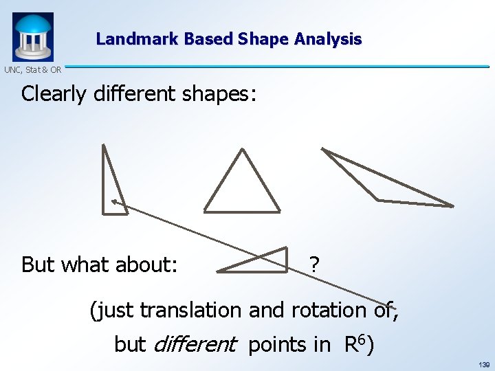
Landmark Based Shape Analysis UNC, Stat & OR Clearly different shapes: But what about: ? (just translation and rotation of, but different points in R 6) 139

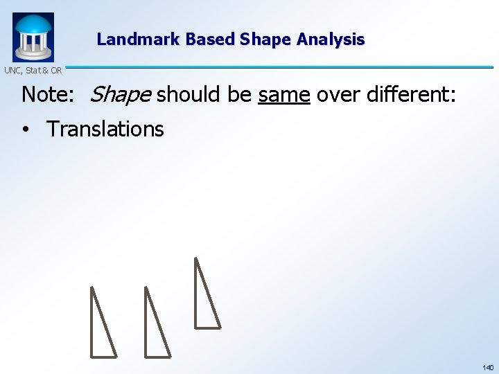
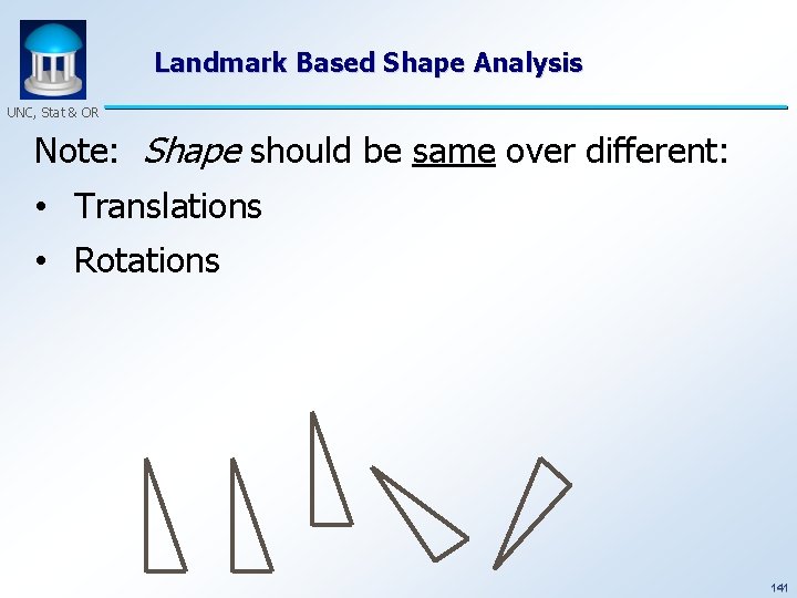
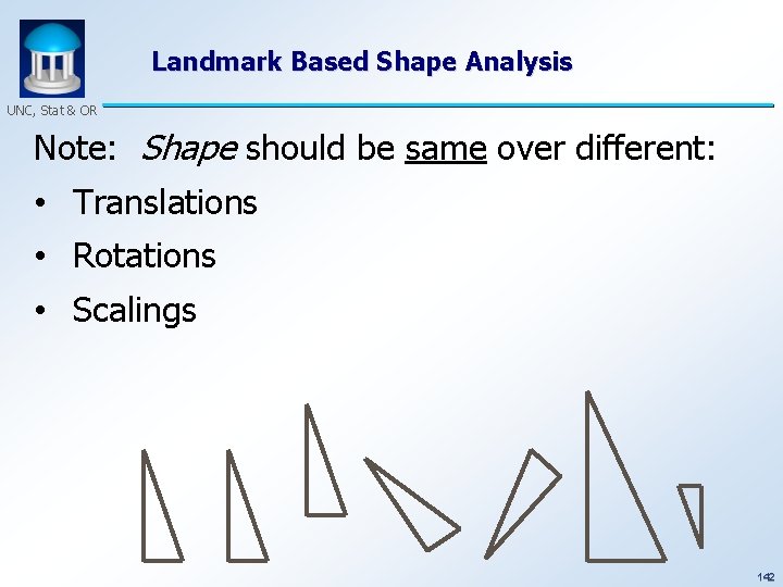
Landmark Based Shape Analysis UNC, Stat & OR Note: Shape should be same over different: • Translations 140

Landmark Based Shape Analysis UNC, Stat & OR Note: Shape should be same over different: • Translations • Rotations 141

Landmark Based Shape Analysis UNC, Stat & OR Note: Shape should be same over different: • Translations • Rotations • Scalings 142

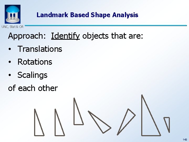
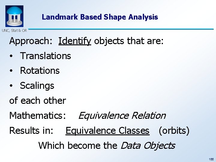
Landmark Based Shape Analysis UNC, Stat & OR Approach: Identify objects that are: • Translations • Rotations • Scalings of each other 143

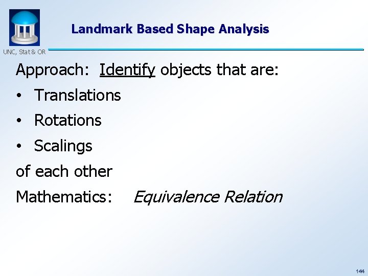
Landmark Based Shape Analysis UNC, Stat & OR Approach: Identify objects that are: • Translations • Rotations • Scalings of each other Mathematics: Equivalence Relation 144

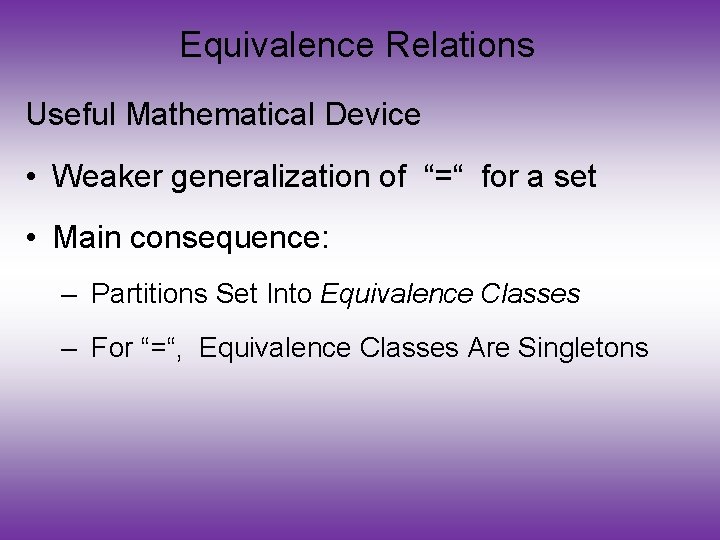
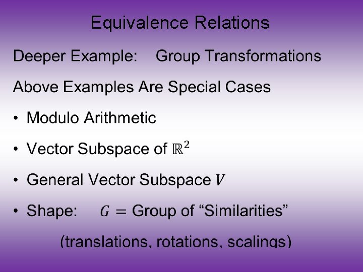
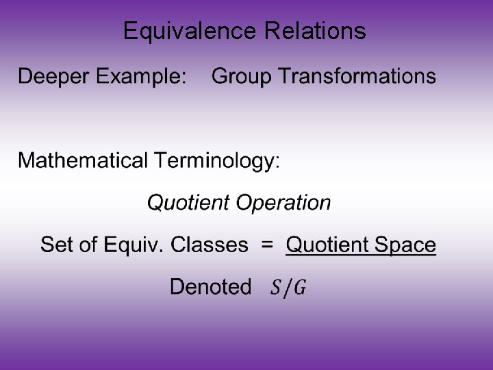
Equivalence Relations Useful Mathematical Device • Weaker generalization of “=“ for a set • Main consequence: – Partitions Set Into Equivalence Classes – For “=“, Equivalence Classes Are Singletons

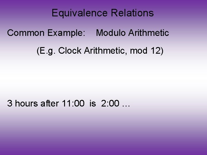
Equivalence Relations Common Example: Modulo Arithmetic (E. g. Clock Arithmetic, mod 12) 3 hours after 11: 00 is 2: 00 …

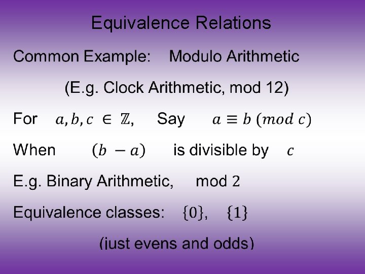
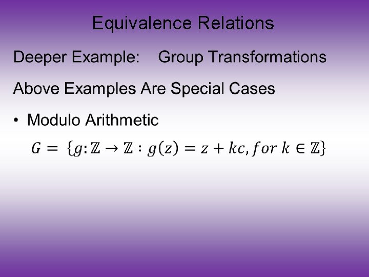
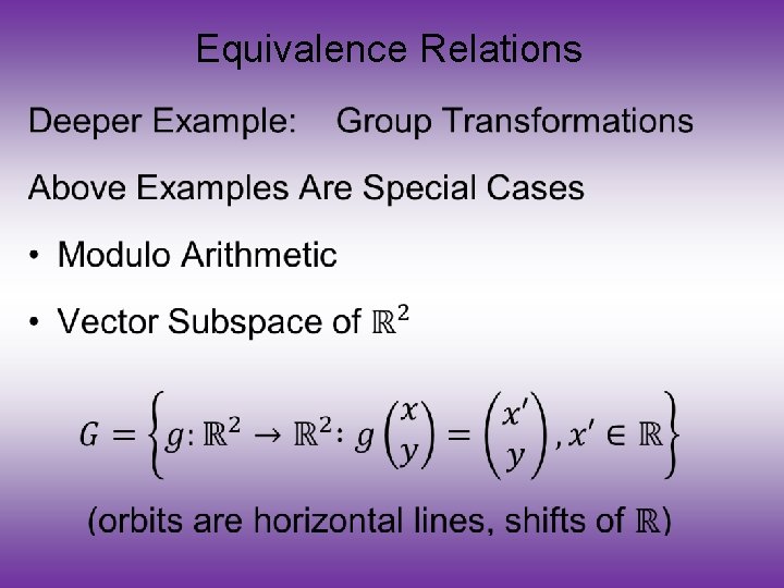
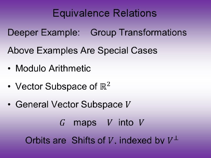
Equivalence Relations •

Equivalence Relations •

Equivalence Relations •

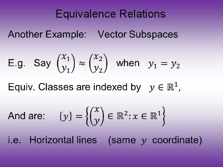
Equivalence Relations •

Equivalence Relations •

Equivalence Relations •

Equivalence Relations •

Equivalence Relations •

Landmark Based Shape Analysis UNC, Stat & OR Approach: Identify objects that are: • Translations • Rotations • Scalings of each other Mathematics: Results in: Equivalence Relation Equivalence Classes (orbits) Which become the Data Objects 155

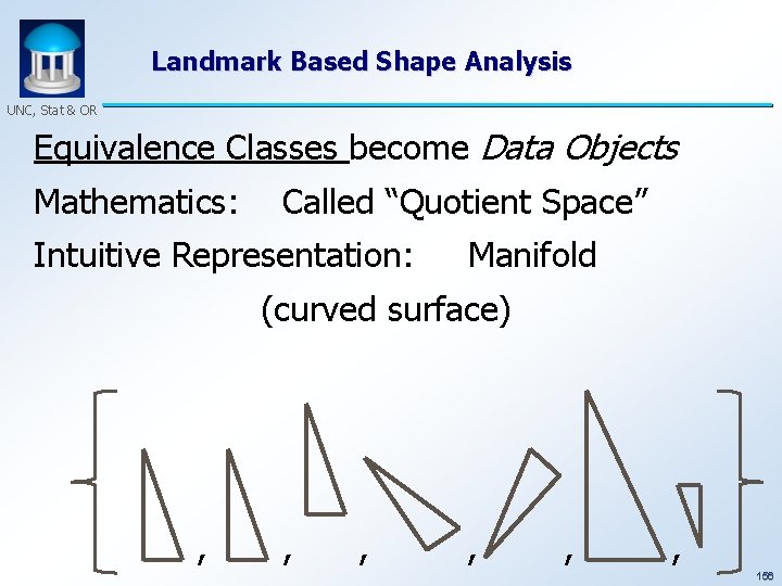
Landmark Based Shape Analysis UNC, Stat & OR Equivalence Classes become Data Objects Mathematics: Called “Quotient Space” Intuitive Representation: Manifold (curved surface) , , , 156

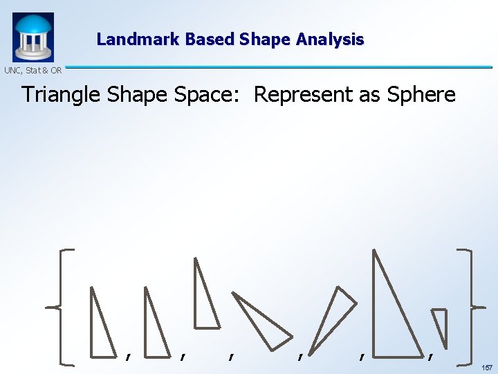
Landmark Based Shape Analysis UNC, Stat & OR Triangle Shape Space: Represent as Sphere , , , 157

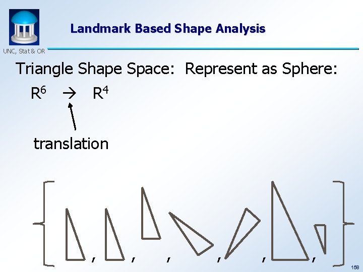
Landmark Based Shape Analysis UNC, Stat & OR Triangle Shape Space: Represent as Sphere: R 6 R 4 translation , , , 158

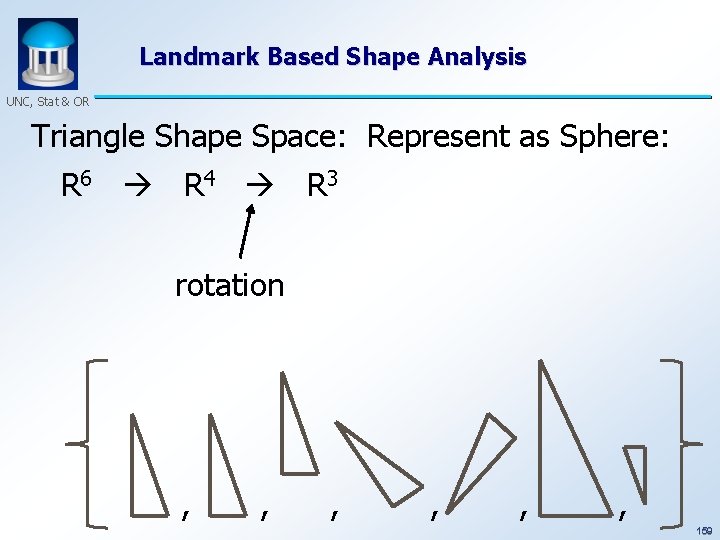
Landmark Based Shape Analysis UNC, Stat & OR Triangle Shape Space: Represent as Sphere: R 6 R 4 R 3 rotation , , , 159

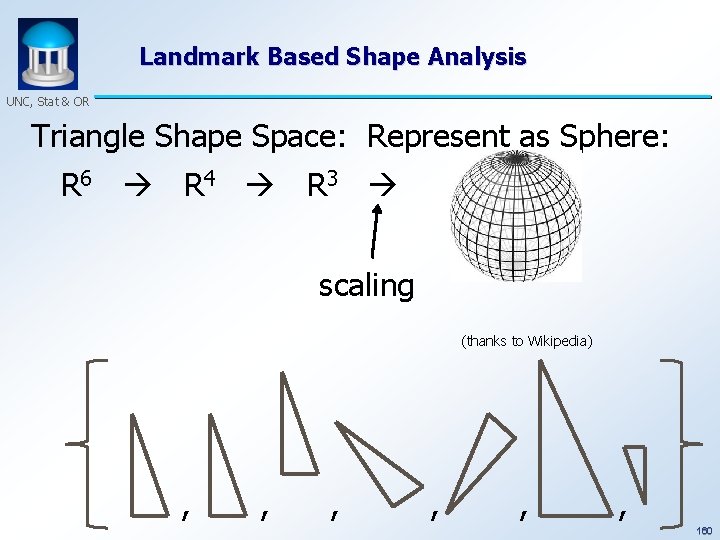
Landmark Based Shape Analysis UNC, Stat & OR Triangle Shape Space: Represent as Sphere: R 6 R 4 R 3 scaling (thanks to Wikipedia) , , , 160

Shapes As Data Objects Common Property of Shape Data Objects: Natural Feature Space is Curved I. e. a Manifold (from Differential Geometry)

Participant Presentation Rui Wang ? ? ?