Clustering EM Algorithm Slides adapted from David Kauchak

Clustering & EM Algorithm Slides adapted from David Kauchak, Sebastian Thrun and Christopher Bishop

Unsupervised Learning • Most of our previous methods were supervised methods • Training Data – Supervised learning: Data <x, y> – Unsupervised Learning: Data x

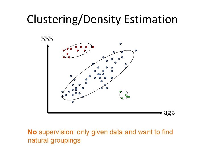
Clustering/Density Estimation $$$ age No supervision: only given data and want to find natural groupings

Unsupervised Learning • Clustering is the most common application for unsupervised learning – Clustering: the process of grouping a set of objects into classes of similar objects • Additionally: learning probabilities/parameters for models – Learn a translation dictionary – Learn a grammar for a language – Learn the social graph

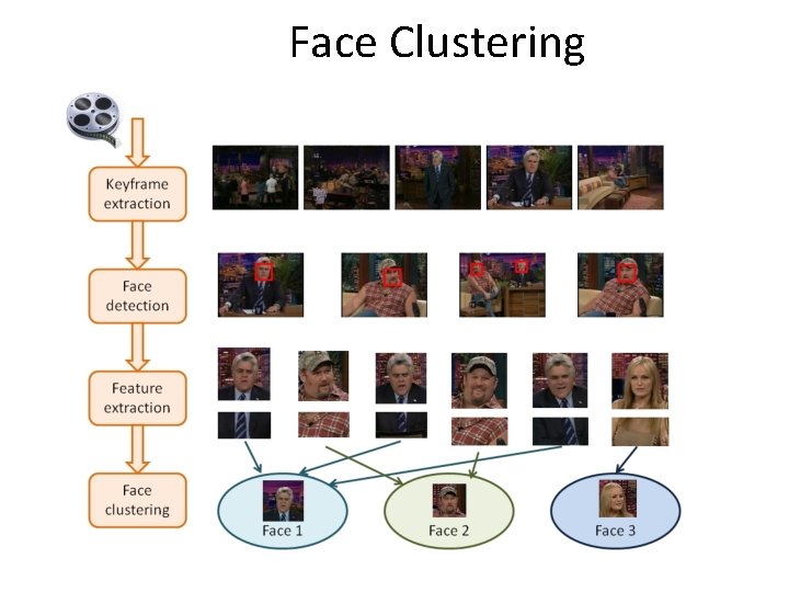
Face Clustering

Google News

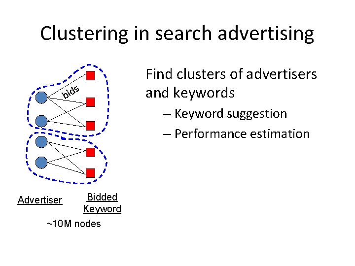
Clustering in search advertising s d i b Find clusters of advertisers and keywords – Keyword suggestion – Performance estimation Bidded Keyword ~10 M nodes Advertiser

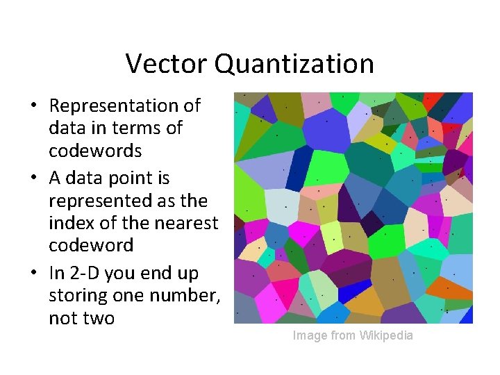
Vector Quantization • Representation of data in terms of codewords • A data point is represented as the index of the nearest codeword • In 2 -D you end up storing one number, not two Image from Wikipedia

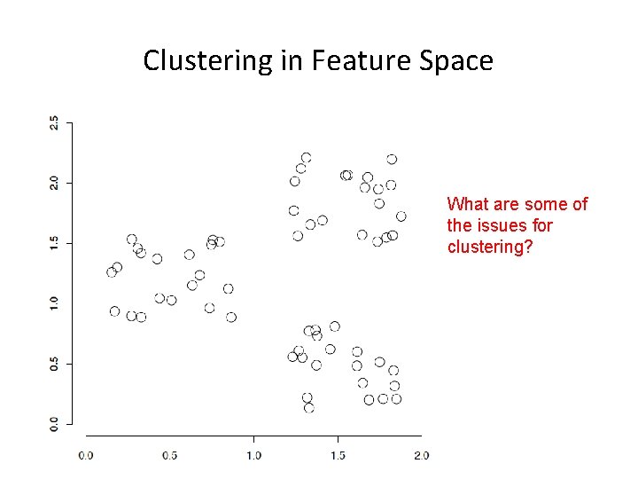
Clustering in Feature Space What are some of the issues for clustering?

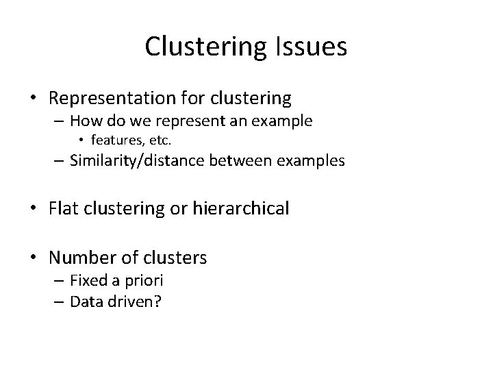
Clustering Issues • Representation for clustering – How do we represent an example • features, etc. – Similarity/distance between examples • Flat clustering or hierarchical • Number of clusters – Fixed a priori – Data driven?

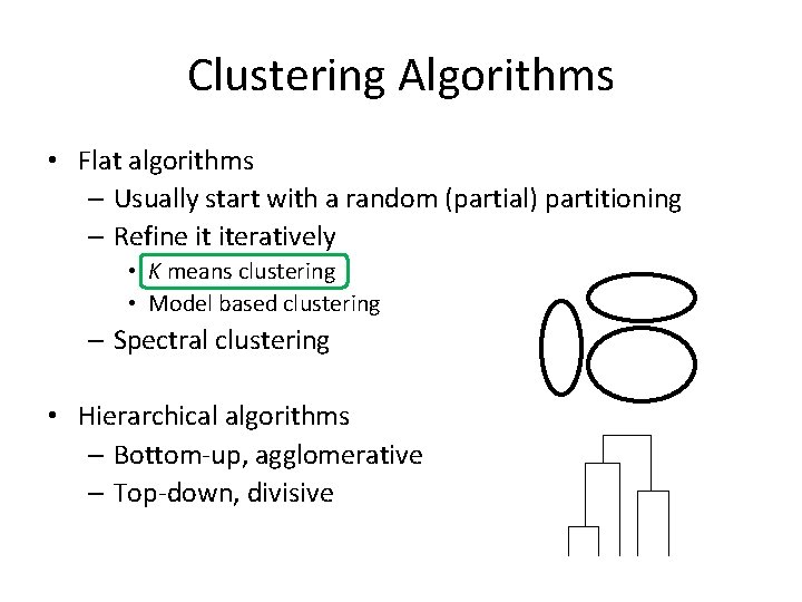
Clustering Algorithms • Flat algorithms – Usually start with a random (partial) partitioning – Refine it iteratively • K means clustering • Model based clustering – Spectral clustering • Hierarchical algorithms – Bottom-up, agglomerative – Top-down, divisive

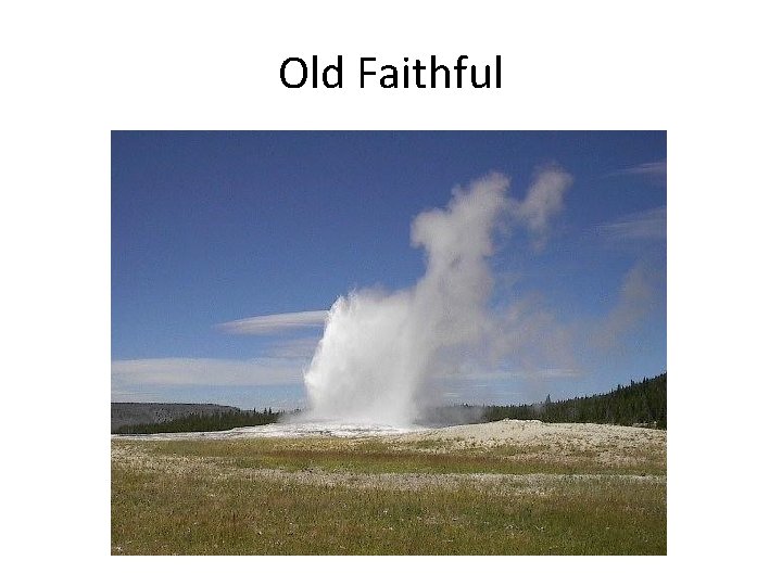
Old Faithful

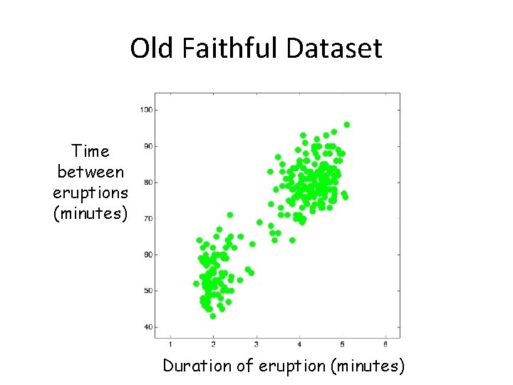
Old Faithful Dataset Time between eruptions (minutes) Duration of eruption (minutes)

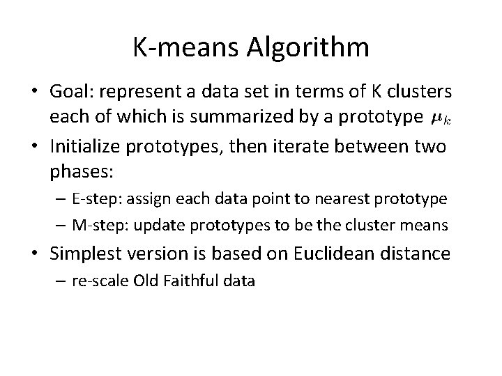
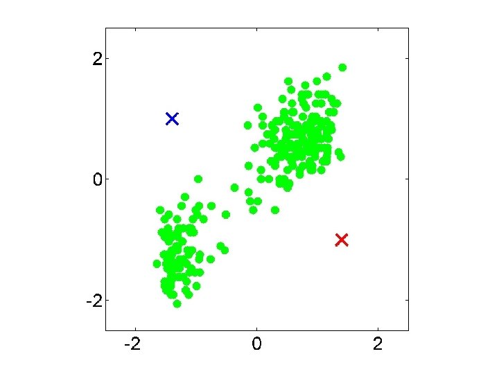
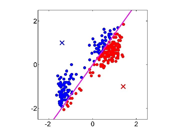
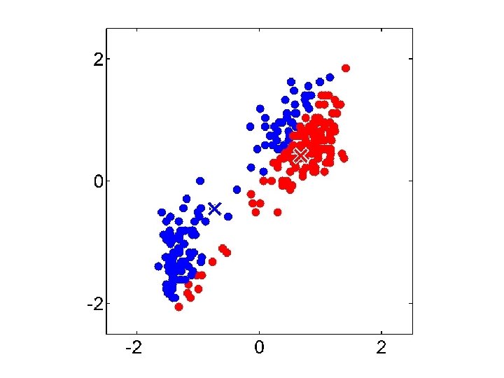
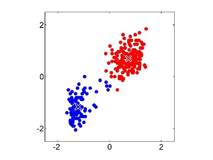
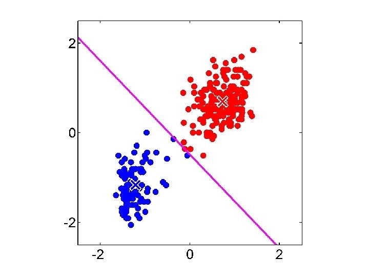
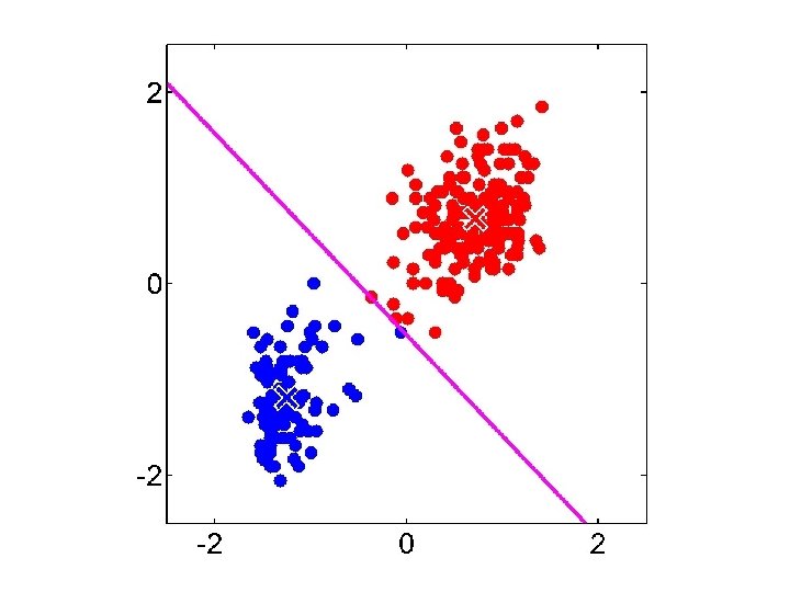
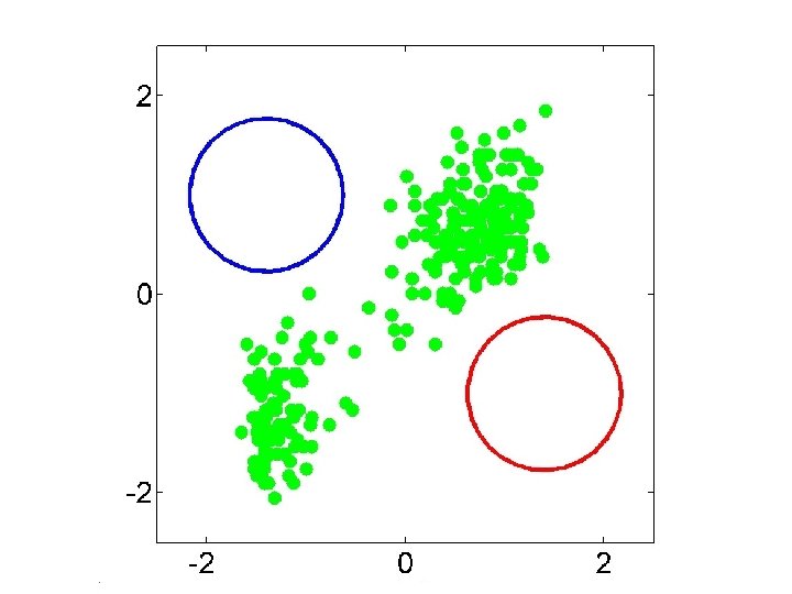
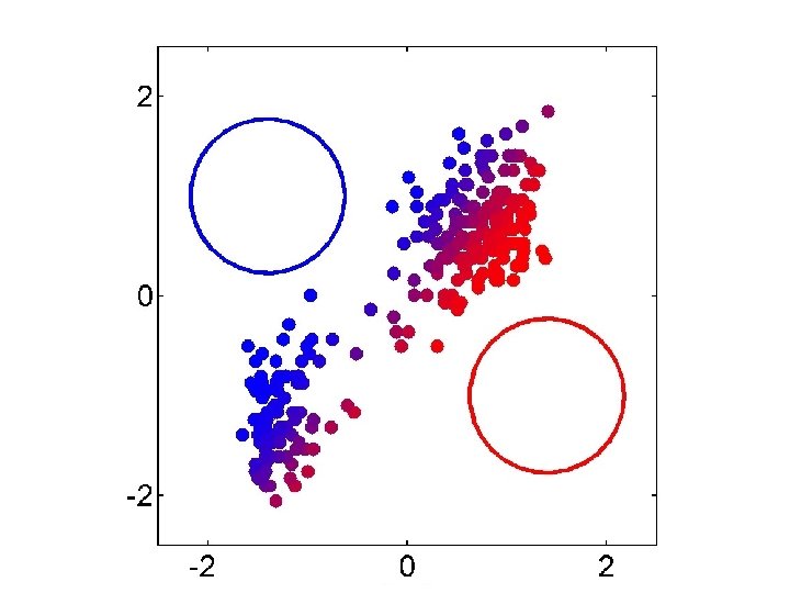
K-means Algorithm • Goal: represent a data set in terms of K clusters each of which is summarized by a prototype • Initialize prototypes, then iterate between two phases: – E-step: assign each data point to nearest prototype – M-step: update prototypes to be the cluster means • Simplest version is based on Euclidean distance – re-scale Old Faithful data

BCS Summer School, Exeter, 2003 Christopher M. Bishop

BCS Summer School, Exeter, 2003 Christopher M. Bishop

BCS Summer School, Exeter, 2003 Christopher M. Bishop

BCS Summer School, Exeter, 2003 Christopher M. Bishop

BCS Summer School, Exeter, 2003 Christopher M. Bishop

BCS Summer School, Exeter, 2003 Christopher M. Bishop

BCS Summer School, Exeter, 2003 Christopher M. Bishop

BCS Summer School, Exeter, 2003 Christopher M. Bishop

BCS Summer School, Exeter, 2003 Christopher M. Bishop

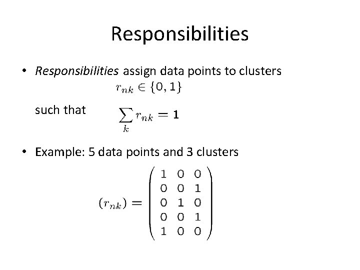
Responsibilities • Responsibilities assign data points to clusters such that • Example: 5 data points and 3 clusters

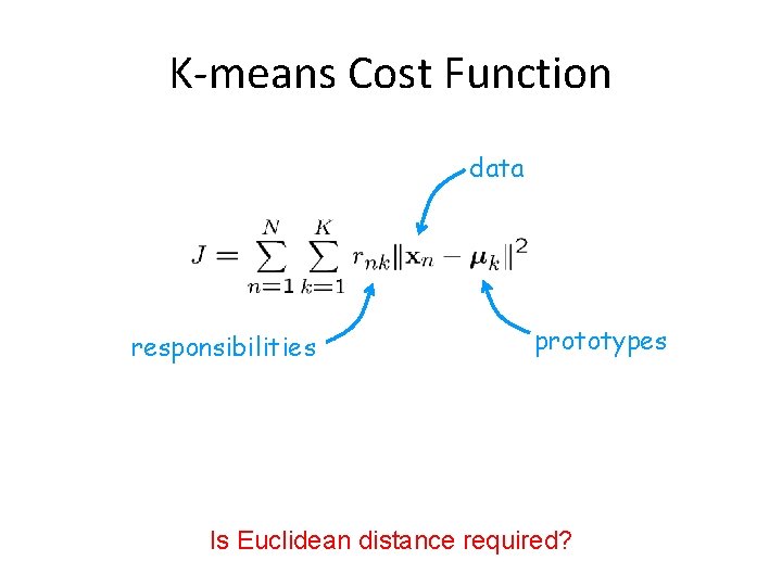
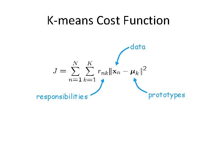
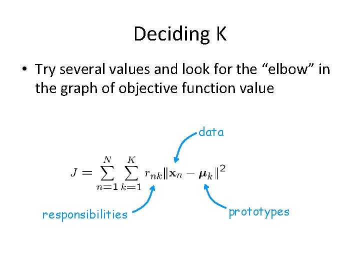
K-means Cost Function data responsibilities prototypes Is Euclidean distance required?

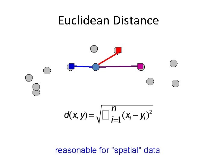
Euclidean Distance reasonable for “spatial” data

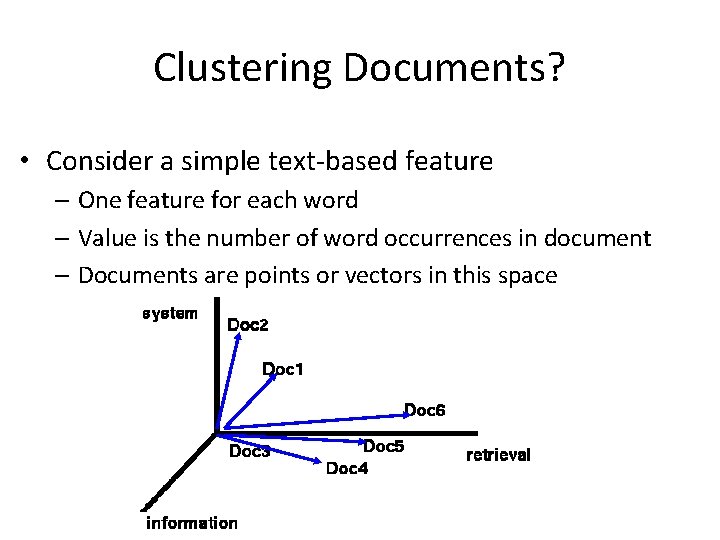
Clustering Documents? • Consider a simple text-based feature – One feature for each word – Value is the number of word occurrences in document – Documents are points or vectors in this space

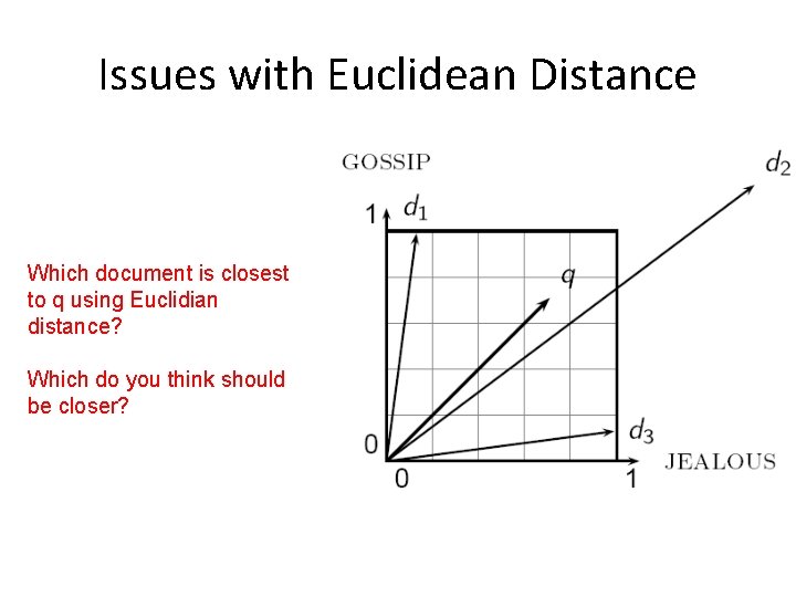
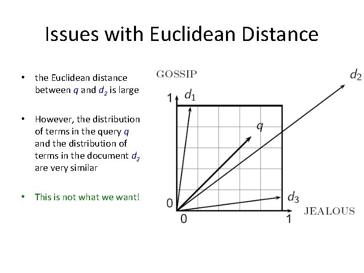
Issues with Euclidean Distance Which document is closest to q using Euclidian distance? Which do you think should be closer?

Issues with Euclidean Distance • the Euclidean distance between q and d 2 is large • However, the distribution of terms in the query q and the distribution of terms in the document d 2 are very similar • This is not what we want!

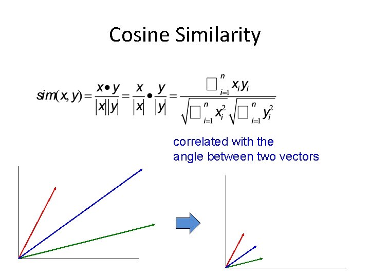
Cosine Similarity correlated with the angle between two vectors

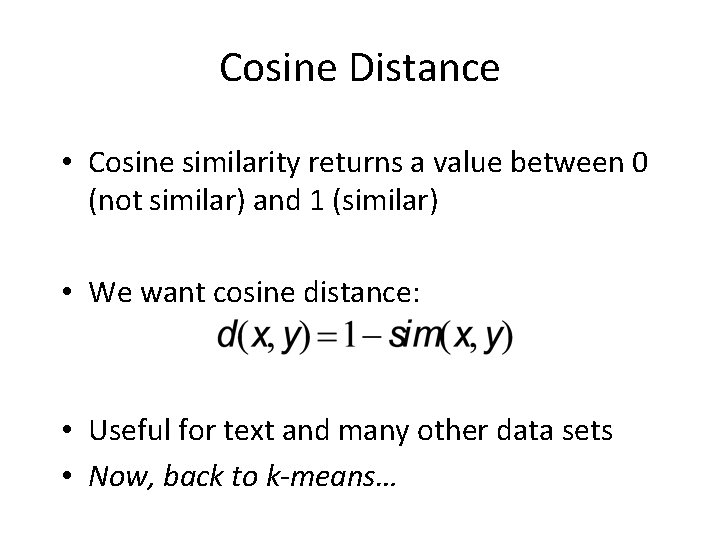
Cosine Distance • Cosine similarity returns a value between 0 (not similar) and 1 (similar) • We want cosine distance: • Useful for text and many other data sets • Now, back to k-means…

K-means Cost Function data responsibilities prototypes

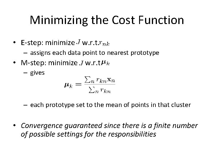
Minimizing the Cost Function • E-step: minimize w. r. t. – assigns each data point to nearest prototype • M-step: minimize w. r. t – gives – each prototype set to the mean of points in that cluster • Convergence guaranteed since there is a finite number of possible settings for the responsibilities

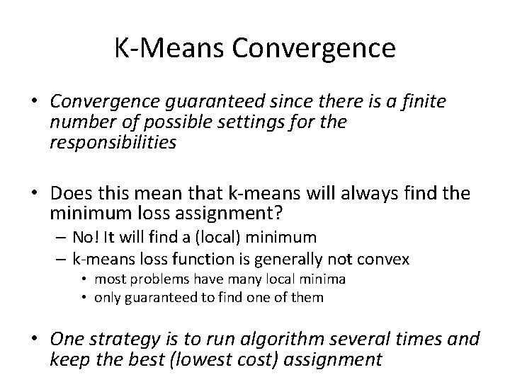
K-Means Convergence • Convergence guaranteed since there is a finite number of possible settings for the responsibilities • Does this mean that k-means will always find the minimum loss assignment? – No! It will find a (local) minimum – k-means loss function is generally not convex • most problems have many local minima • only guaranteed to find one of them • One strategy is to run algorithm several times and keep the best (lowest cost) assignment

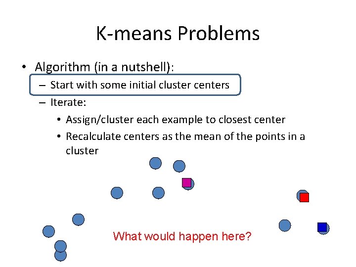
K-means Problems • Algorithm (in a nutshell): – Start with some initial cluster centers – Iterate: • Assign/cluster each example to closest center • Recalculate centers as the mean of the points in a cluster What would happen here?

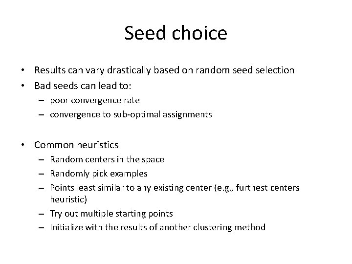
Seed choice • Results can vary drastically based on random seed selection • Bad seeds can lead to: – poor convergence rate – convergence to sub-optimal assignments • Common heuristics – Random centers in the space – Randomly pick examples – Points least similar to any existing center (e. g. , furthest centers heuristic) – Try out multiple starting points – Initialize with the results of another clustering method

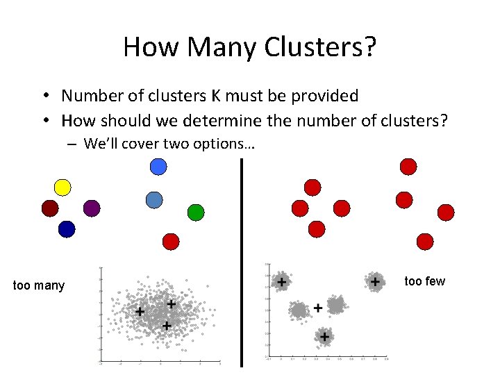
How Many Clusters? • Number of clusters K must be provided • How should we determine the number of clusters? – We’ll cover two options… too many too few

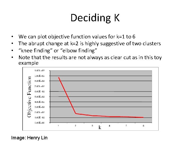
Deciding K • Try several values and look for the “elbow” in the graph of objective function value data responsibilities prototypes

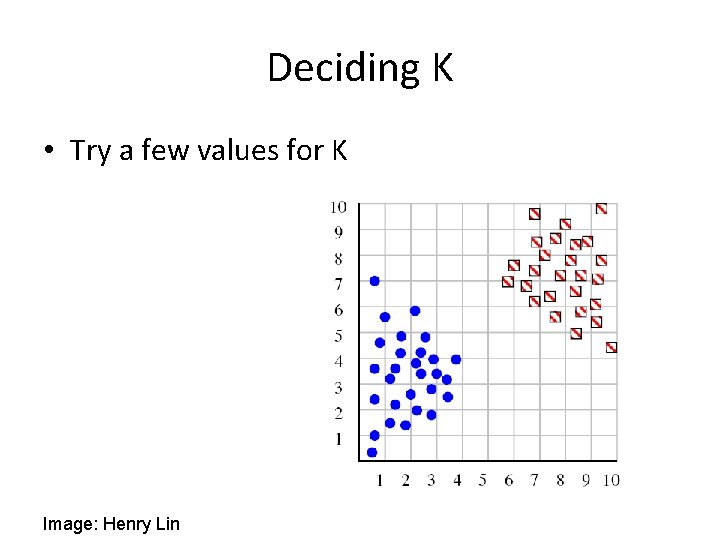
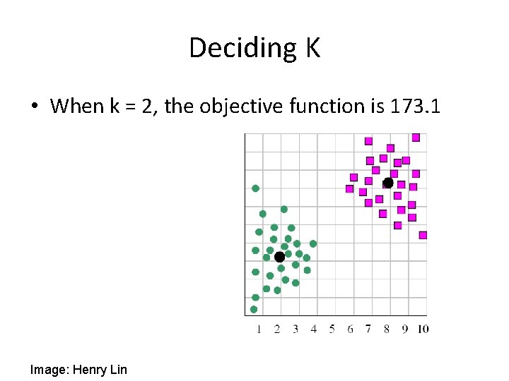
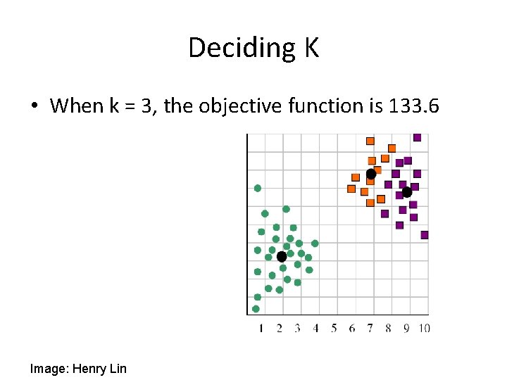
Deciding K • Try a few values for K Image: Henry Lin

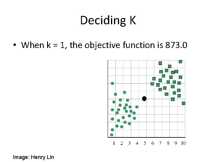
Deciding K • When k = 1, the objective function is 873. 0 Image: Henry Lin

Deciding K • When k = 2, the objective function is 173. 1 Image: Henry Lin

Deciding K • When k = 3, the objective function is 133. 6 Image: Henry Lin

Deciding K • • We can plot objective function values for k=1 to 6 The abrupt change at k=2 is highly suggestive of two clusters “knee finding” or “elbow finding” Note that the results are not always as clear cut as in this toy example Image: Henry Lin

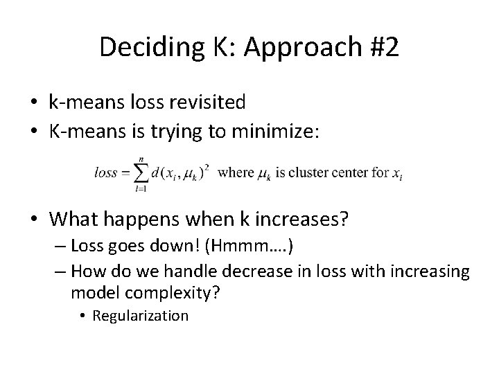
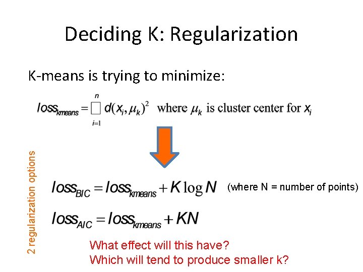
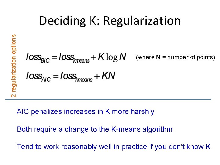
Deciding K: Approach #2 • k-means loss revisited • K-means is trying to minimize: • What happens when k increases? – Loss goes down! (Hmmm…. ) – How do we handle decrease in loss with increasing model complexity? • Regularization

Deciding K: Regularization 2 regularization options K-means is trying to minimize: (where N = number of points) What effect will this have? Which will tend to produce smaller k?

2 regularization options Deciding K: Regularization (where N = number of points) AIC penalizes increases in K more harshly Both require a change to the K-means algorithm Tend to work reasonably well in practice if you don’t know K

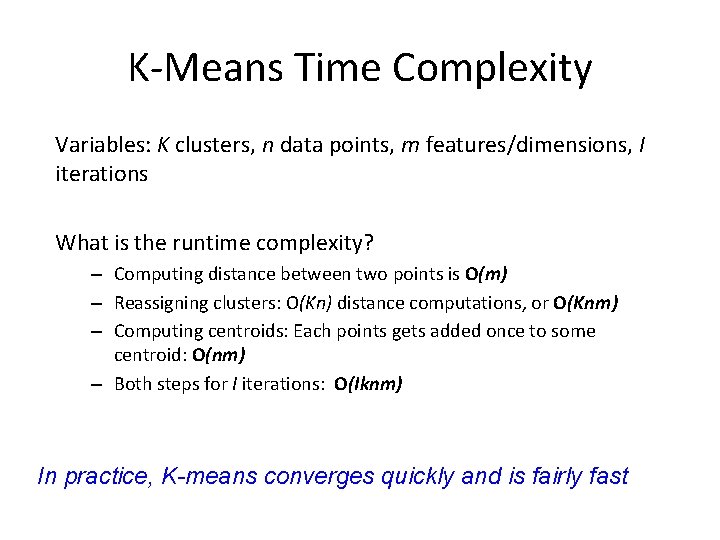
K-Means Time Complexity Variables: K clusters, n data points, m features/dimensions, I iterations What is the runtime complexity? – Computing distance between two points is O(m) – Reassigning clusters: O(Kn) distance computations, or O(Knm) – Computing centroids: Each points gets added once to some centroid: O(nm) – Both steps for I iterations: O(Iknm) In practice, K-means converges quickly and is fairly fast

What Is A Good Clustering Assignment? • A good clustering will produce: – High intra-class (i. e. , intra-cluster) similarity – Low inter-class similarity • How should we evaluate clustering? – Common approach: use labeled data • Cluster input data (without labels) • Check to see if clusters reproduce class partitions

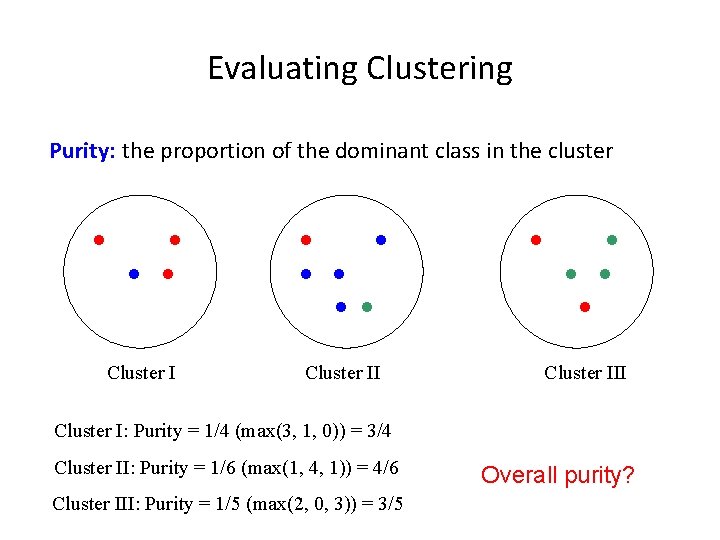
Evaluating Clustering Purity: the proportion of the dominant class in the cluster Cluster III Cluster I: Purity = 1/4 (max(3, 1, 0)) = 3/4 Cluster II: Purity = 1/6 (max(1, 4, 1)) = 4/6 Cluster III: Purity = 1/5 (max(2, 0, 3)) = 3/5 Overall purity?

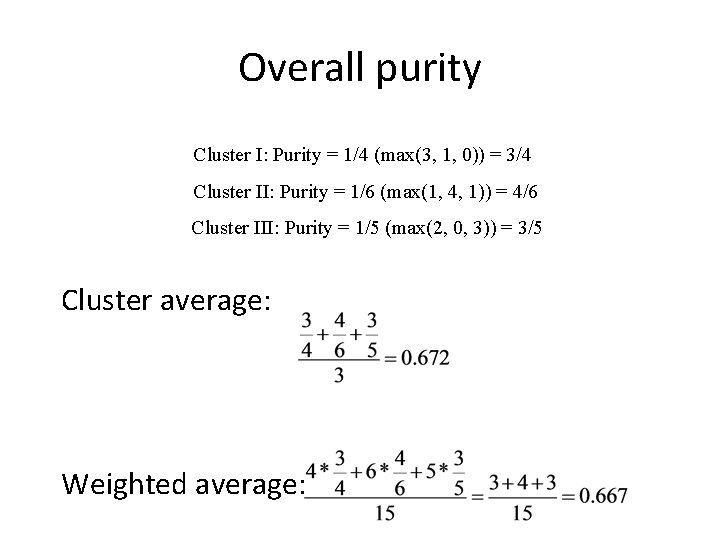
Overall purity Cluster I: Purity = 1/4 (max(3, 1, 0)) = 3/4 Cluster II: Purity = 1/6 (max(1, 4, 1)) = 4/6 Cluster III: Purity = 1/5 (max(2, 0, 3)) = 3/5 Cluster average: Weighted average:

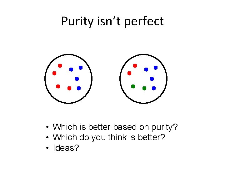
Purity isn’t perfect • Which is better based on purity? • Which do you think is better? • Ideas?

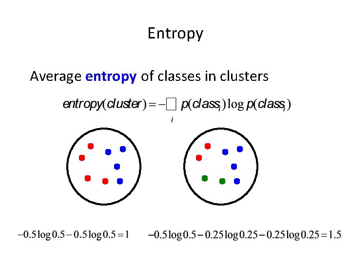
Entropy Average entropy of classes in clusters

K-means Remaining Issues • The last two issues are not as obvious • K-Means assumes a spherical distribution • Hard assignments – Small change in data point can switch it to a different cluster • Can both be addressed with Gaussian Mixture Models…

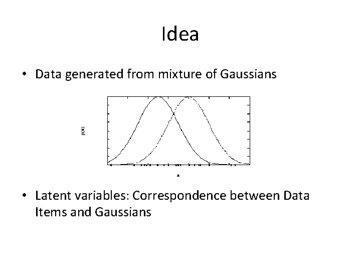
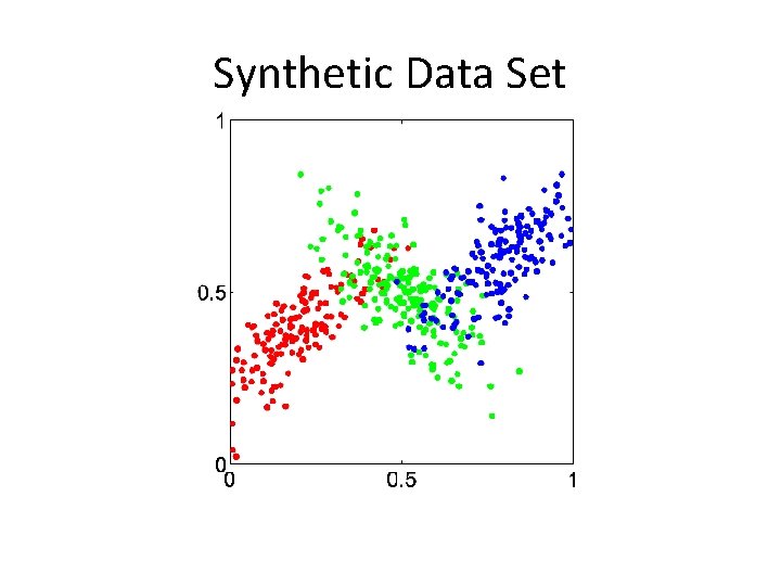
Idea • Data generated from mixture of Gaussians • Latent variables: Correspondence between Data Items and Gaussians

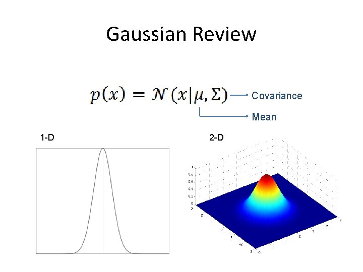
Gaussian Review Covariance Mean 1 -D 2 -D

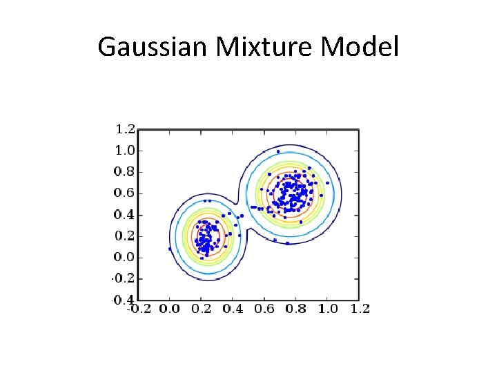
Gaussian Mixture Model

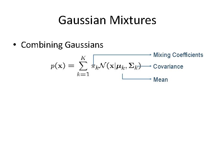
Gaussian Mixtures • Combining Gaussians Mixing Coefficients Covariance Mean

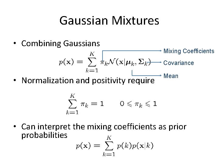
Gaussian Mixtures • Combining Gaussians Mixing Coefficients Covariance • Normalization and positivity require Mean • Can interpret the mixing coefficients as prior probabilities

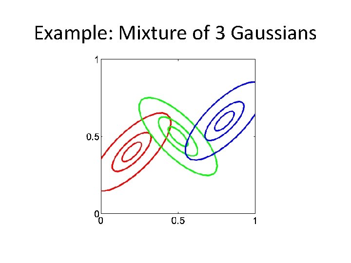
Example: Mixture of 3 Gaussians

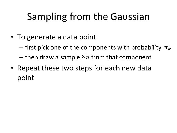
Sampling from the Gaussian • To generate a data point: – first pick one of the components with probability – then draw a sample from that component • Repeat these two steps for each new data point

Synthetic Data Set

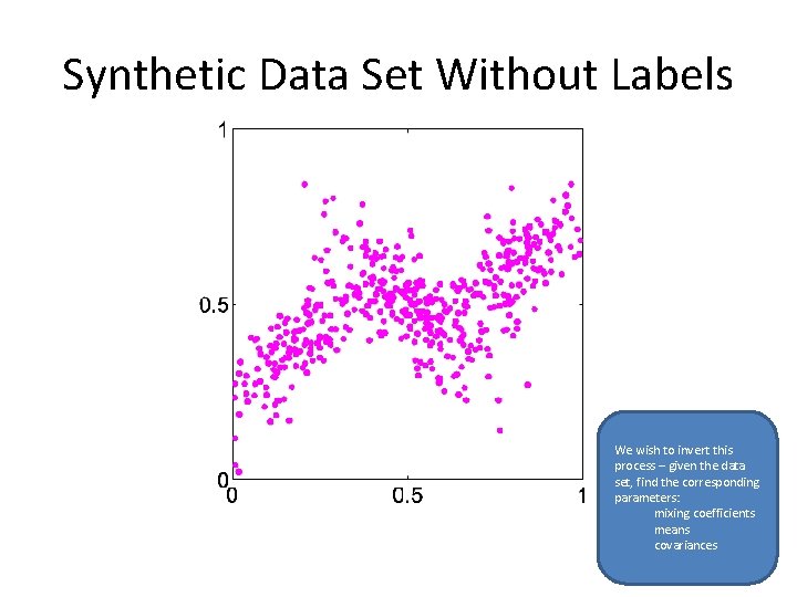
Synthetic Data Set Without Labels We wish to invert this process – given the data set, find the corresponding parameters: mixing coefficients means covariances

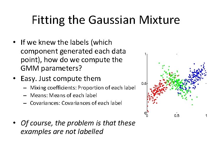
Fitting the Gaussian Mixture • If we knew the labels (which component generated each data point), how do we compute the GMM parameters? • Easy. Just compute them – Mixing coefficients: Proportion of each label – Means: Means of each label – Covariances: Covariances of each label • Of course, the problem is that these examples are not labelled

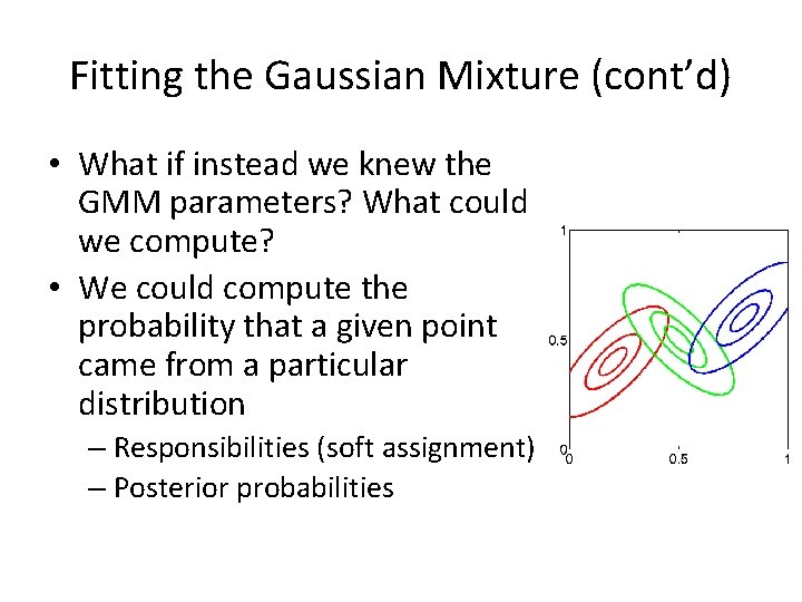
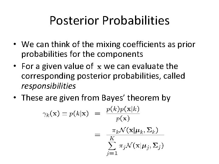
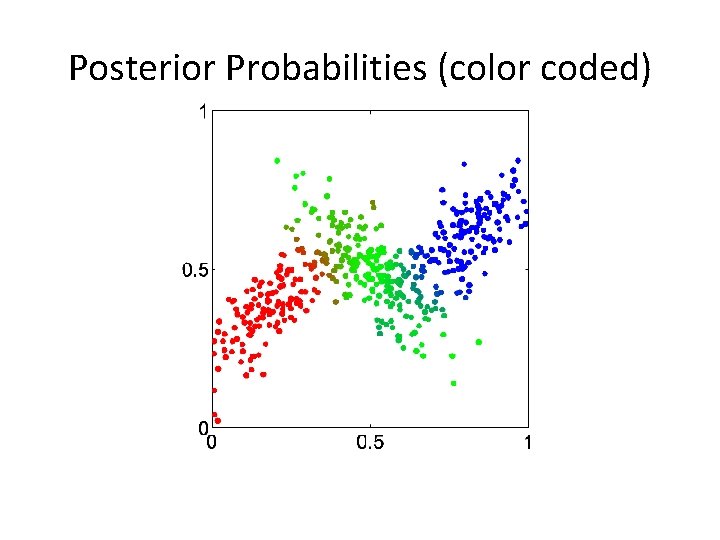
Fitting the Gaussian Mixture (cont’d) • What if instead we knew the GMM parameters? What could we compute? • We could compute the probability that a given point came from a particular distribution – Responsibilities (soft assignment) – Posterior probabilities

Posterior Probabilities • We can think of the mixing coefficients as prior probabilities for the components • For a given value of we can evaluate the corresponding posterior probabilities, called responsibilities • These are given from Bayes’ theorem by

Posterior Probabilities (color coded)

The EM Algorithm • Expectation-Maximization – Method frequently referenced throughout field of statistics – Term coined in 1977 paper by Arthur Dempster, Nan Laird, and Donald Rubin • Great for problems such as: – If only I knew the value of certain variables, I could compute the right ML hypothesis – If only I knew the right ML hypothesis, I could immediately compute a probability distribution for those variables • Chicken-and-egg problems • Used when some features are not observable – We call these features latent variables

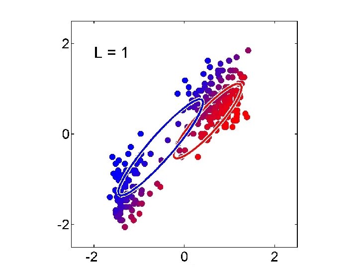
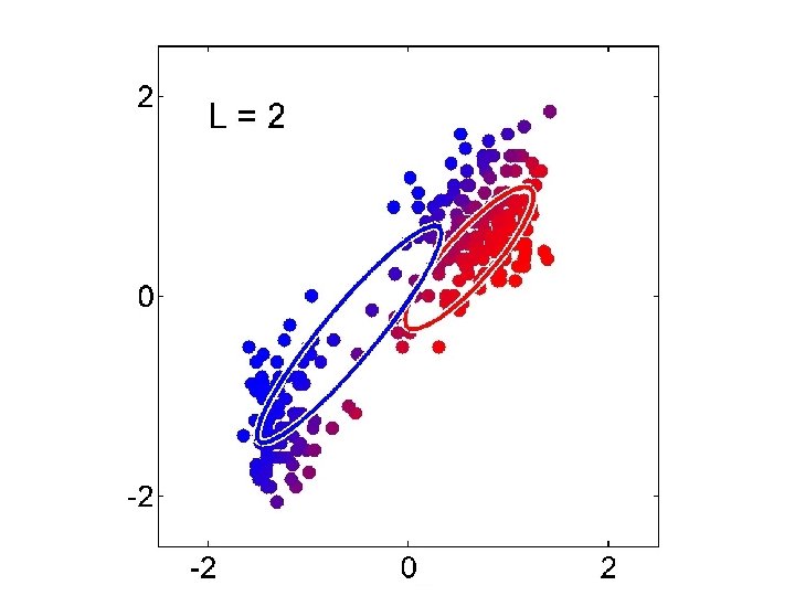
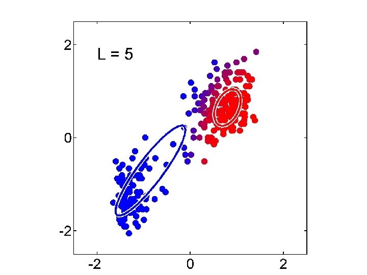
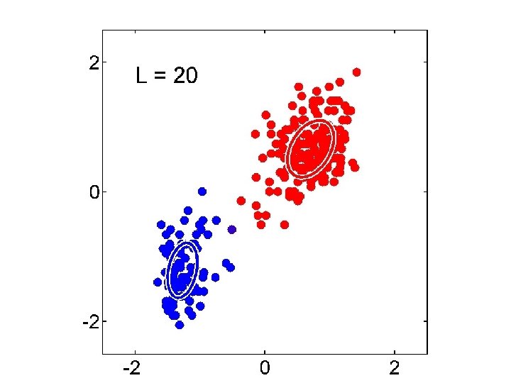
EM Algorithm • The solutions are not closed form since they are coupled • Suggests an iterative scheme for solving them: – Make initial guesses for the parameters – Alternate between the following two stages: 1. E-step: evaluate responsibilities 2. M-step: update parameters using ML results

BCS Summer School, Exeter, 2003 Christopher M. Bishop

BCS Summer School, Exeter, 2003 Christopher M. Bishop

BCS Summer School, Exeter, 2003 Christopher M. Bishop

BCS Summer School, Exeter, 2003 Christopher M. Bishop

BCS Summer School, Exeter, 2003 Christopher M. Bishop

BCS Summer School, Exeter, 2003 Christopher M. Bishop

Gaussian Mixture Model vs. K-means • More complex model can better capture the shape of clusters • GMM allows for soft clustering • GMM typically converges more slowly than Kmeans • GMM initialization often done with K-means

EM Algorithm • EM is a general purpose approach for training a model when you don’t have labels – Not just for clustering! • One of the most general-purpose unsupervised approaches – – – Training HMMs (Baum-Welch algorithm) Learning probabilities for Bayesian networks Learning word alignments for language translation Learning Twitter friend network Genetics Finance

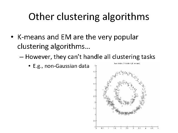
Other clustering algorithms • K-means and EM are the very popular clustering algorithms… – However, they can’t handle all clustering tasks • E. g. , non-Gaussian data

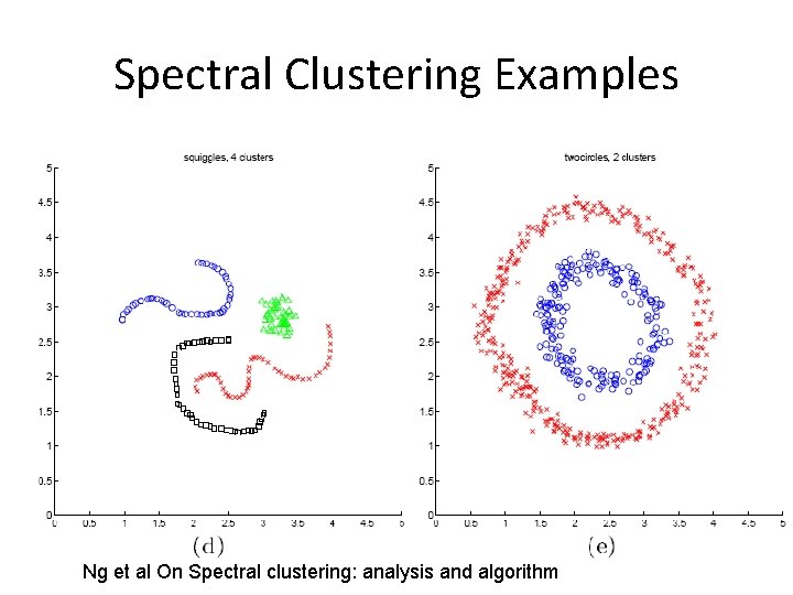
Spectral Clustering Examples Ng et al On Spectral clustering: analysis and algorithm