Clustering different types of data Pasi Frnti 21

Clustering different types of data Pasi Fränti 21. 3. 2017

Data types • • • Numeric Binary Categorical Text Time series

Part I: Numeric data

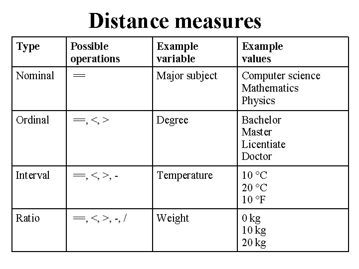
Distance measures Type Possible operations Example variable Example values Nominal == Major subject Computer science Mathematics Physics Ordinal ==, <, > Degree Bachelor Master Licentiate Doctor Interval ==, <, >, - Temperature 10 °C 20 °C 10 °F Ratio ==, <, >, -, / Weight 0 kg 10 kg 20 kg

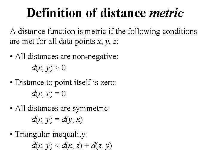
Definition of distance metric A distance function is metric if the following conditions are met for all data points x, y, z: • All distances are non-negative: d(x, y) ≥ 0 • Distance to point itself is zero: d(x, x) = 0 • All distances are symmetric: d(x, y) = d(y, x) • Triangular inequality: d(x, y) d(x, z) + d(z, y)

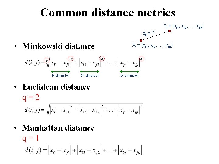
Common distance metrics Xj = (xj 1, xj 2, …, xjp) dij = ? • Minkowski distance 1 st dimension 2 nd dimension • Euclidean distance q = 2 • Manhattan distance q = 1 Xi = (xi 1, xi 2, …, xip) pth dimension

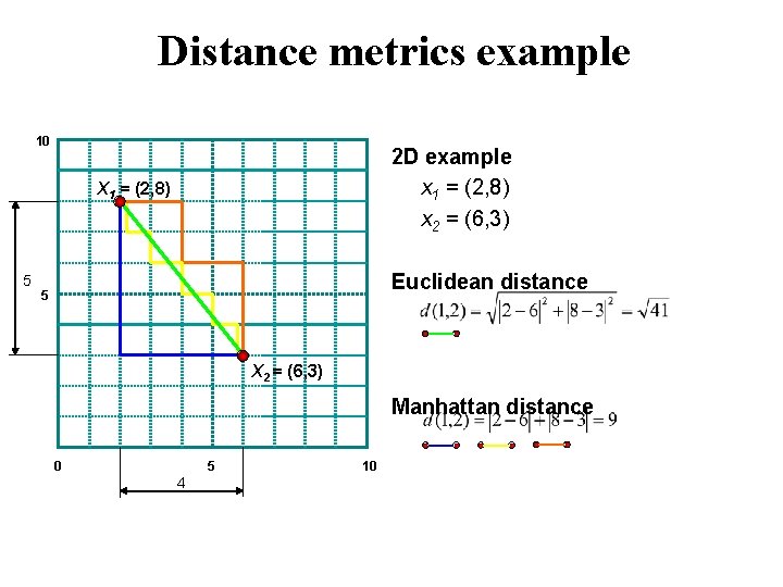
Distance metrics example 10 2 D example x 1 = (2, 8) x 2 = (6, 3) X 1 = (2, 8) 5 Euclidean distance 5 X 2 = (6, 3) Manhattan distance 0 5 4 10

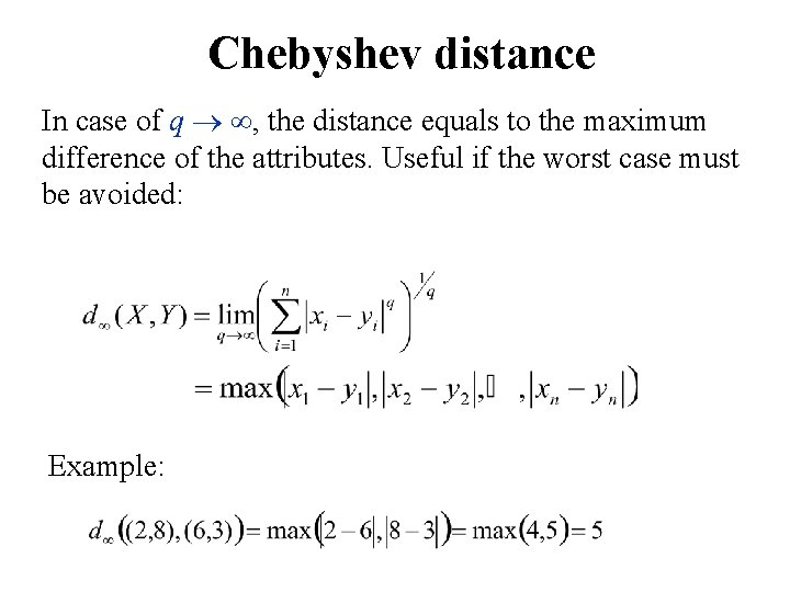
Chebyshev distance In case of q , the distance equals to the maximum difference of the attributes. Useful if the worst case must be avoided: Example:

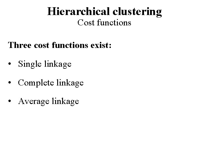
Hierarchical clustering Cost functions Three cost functions exist: • Single linkage • Complete linkage • Average linkage

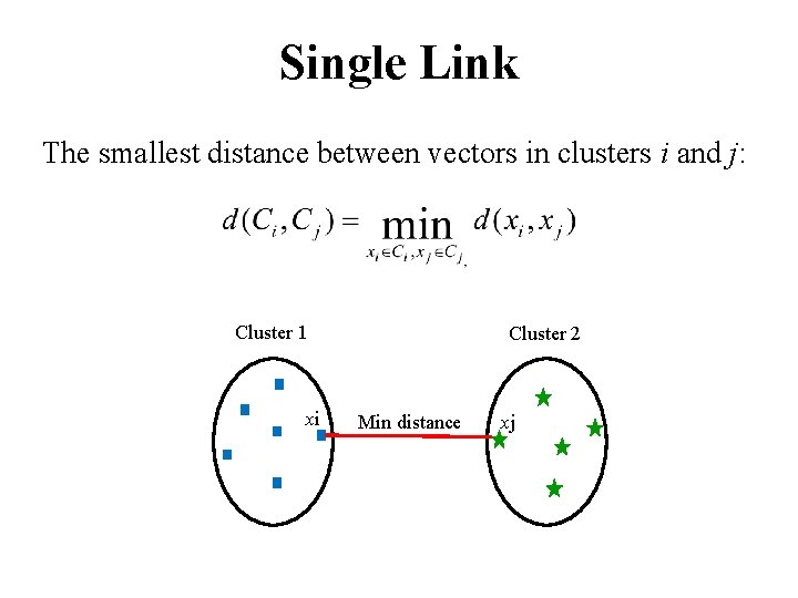
Single Link The smallest distance between vectors in clusters i and j: Cluster 1 xi Cluster 2 Min distance xj

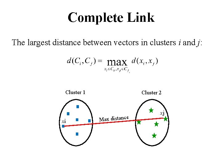
Complete Link The largest distance between vectors in clusters i and j: Cluster 1 xi Cluster 2 Max distance xj

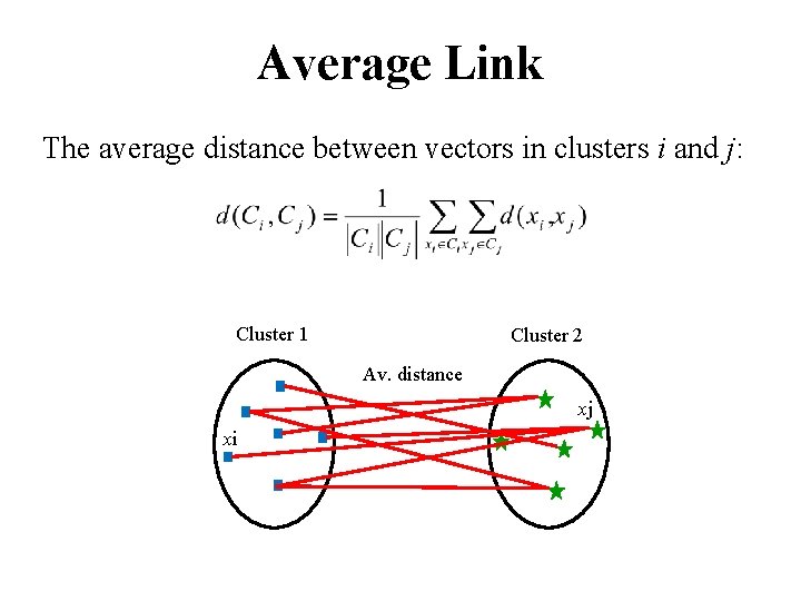
Average Link The average distance between vectors in clusters i and j: Cluster 1 Cluster 2 Av. distance xj xi

Cost function example [Theodoridis, Koutroumbas, 2006] 1 Data Set x 1 1. 1 x 2 1. 2 x 3 1. 3 x 4 1. 4 x 5 Single Link: x 1 x 2 x 3 x 4 x 5 1. 5 x 6 x 7 Complete Link: x 6 x 7 x 1 x 2 x 3 x 4 x 5 x 6 x 7

Part II: Binary data

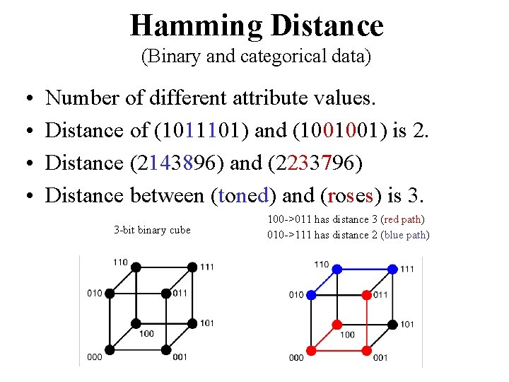
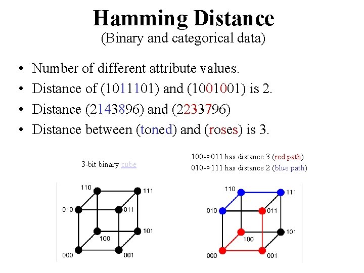
Hamming Distance (Binary and categorical data) • • Number of different attribute values. Distance of (1011101) and (1001001) is 2. Distance (2143896) and (2233796) Distance between (toned) and (roses) is 3. 3 -bit binary cube 100 ->011 has distance 3 (red path) 010 ->111 has distance 2 (blue path)

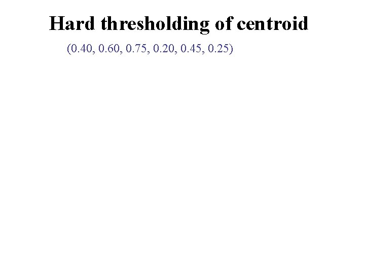
Hard thresholding of centroid (0. 40, 0. 60, 0. 75, 0. 20, 0. 45, 0. 25)

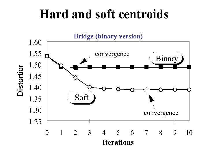
Hard and soft centroids Bridge (binary version)

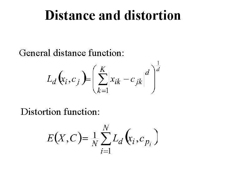
Distance and distortion General distance function: Distortion function:

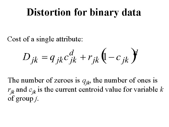
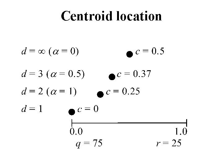
Distortion for binary data Cost of a single attribute: The number of zeroes is qjk, the number of ones is rjk and cjk is the current centroid value for variable k of group j.

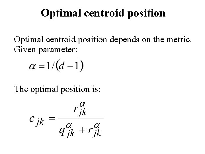
Optimal centroid position depends on the metric. Given parameter: The optimal position is:

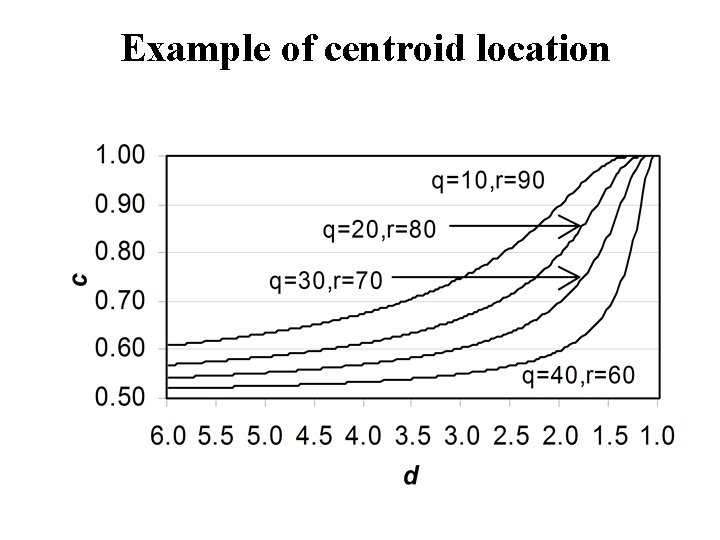
Example of centroid location

Centroid location

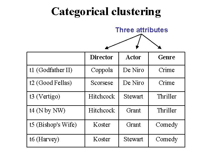
Categorical clustering Three attributes Director Actor Genre t 1 (Godfather II) Coppola De Niro Crime t 2 (Good Fellas) Scorsese De Niro Crime t 3 (Vertigo) Hitchcock Stewart Thriller t 4 (N by NW) Hitchcock Grant Thriller t 5 (Bishop's Wife) Koster Grant Comedy t 6 (Harvey) Koster Stewart Comedy

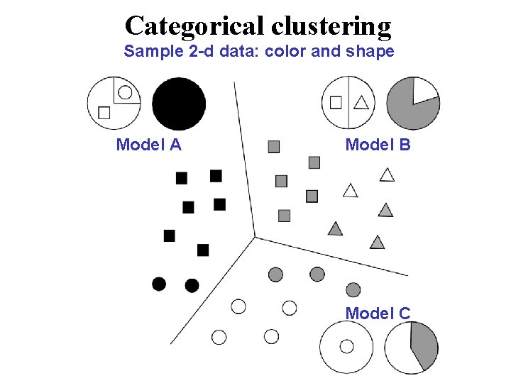
Categorical clustering Sample 2 -d data: color and shape Model A Model B Model C

Hamming Distance (Binary and categorical data) • • Number of different attribute values. Distance of (1011101) and (1001001) is 2. Distance (2143896) and (2233796) Distance between (toned) and (roses) is 3. 3 -bit binary cube 100 ->011 has distance 3 (red path) 010 ->111 has distance 2 (blue path)

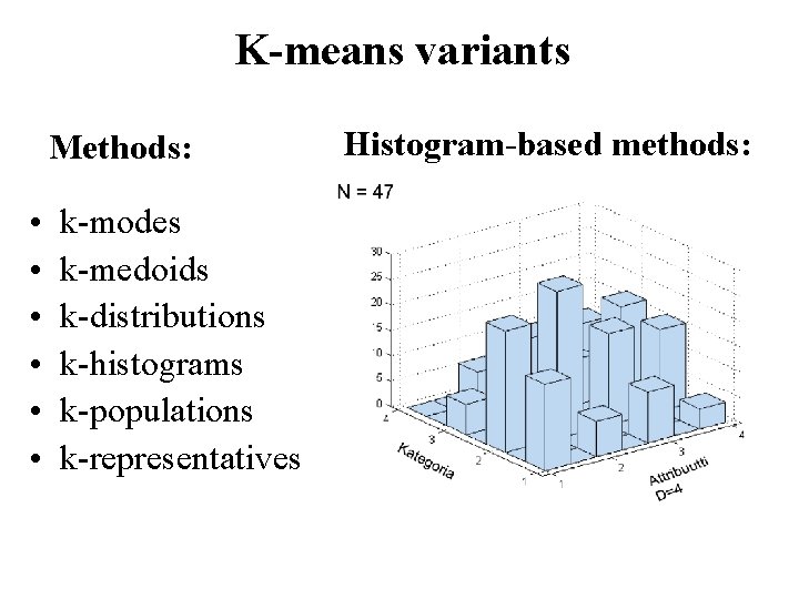
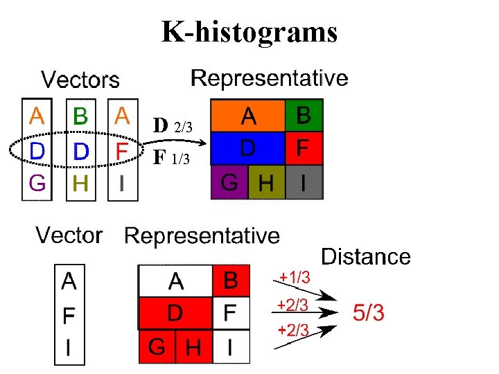
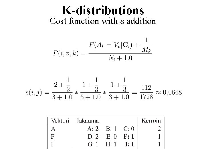
K-means variants Methods: • • • k-modes k-medoids k-distributions k-histograms k-populations k-representatives Histogram-based methods:

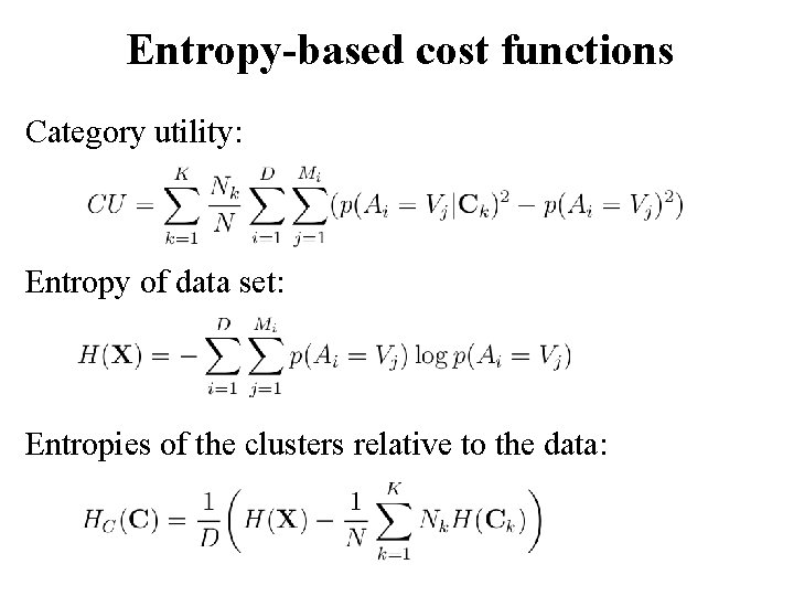
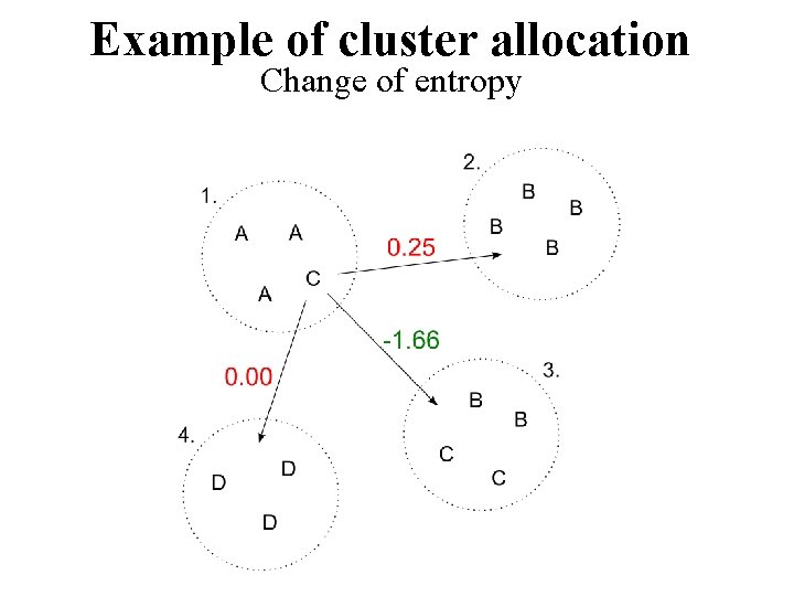
Entropy-based cost functions Category utility: Entropy of data set: Entropies of the clusters relative to the data:

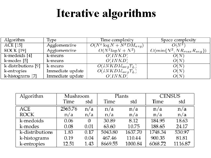
Iterative algorithms

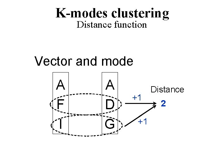
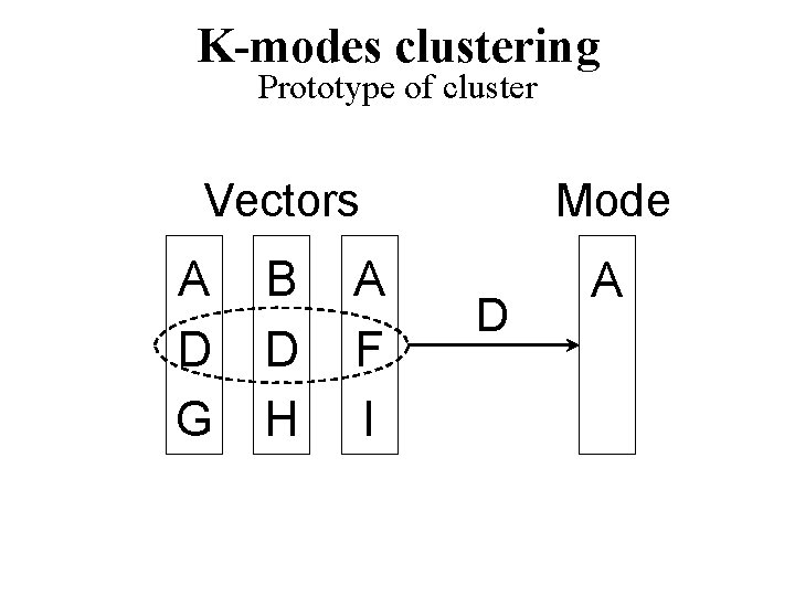
K-modes clustering Distance function Vector and mode A F I A D G +1 +1 Distance 2

K-modes clustering Prototype of cluster Vectors A D G B D H A F I Mode D A

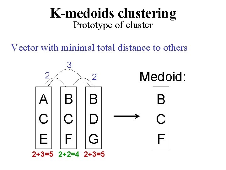
K-medoids clustering Prototype of cluster Vector with minimal total distance to others 3 2 A C E B C F 2 Medoid: B D G B C F 2+3=5 2+2=4 2+3=5

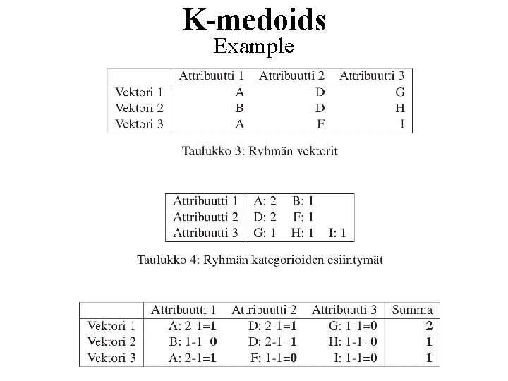
K-medoids Example

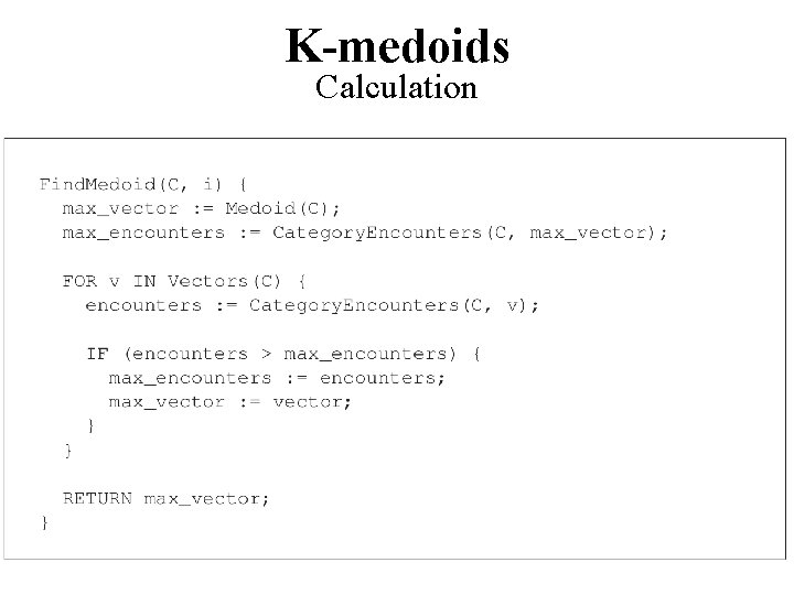
K-medoids Calculation

K-histograms D 2/3 F 1/3

K-distributions Cost function with ε addition

Example of cluster allocation Change of entropy

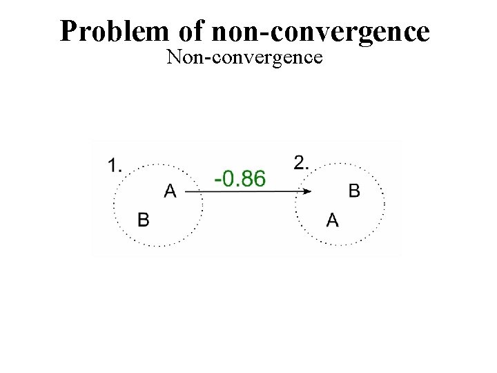
Problem of non-convergence Non-convergence

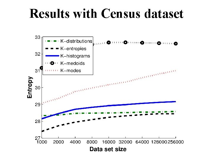
Results with Census dataset

Literature Modified k-modes + k-histograms: M. Ng, M. J. Li, J. Z. Huang and Z. He, On the Impact of Dissimilarity Measure in k-Modes Clustering Algorithm, IEEE Trans. on Pattern Analysis and Machine Intelligence, 29 (3), 503 -507, March, 2007. ACE: K. Chen and L. Liu, The “Best k'' for entropy-based categorical data clustering, Int. Conf. on Scientific and Statistical Database Management (SSDBM'2005), pp. 253 -262, Berkeley, USA, 2005. ROCK: S. Guha, R. Rastogi and K. Shim, “Rock: A robust clustering algorithm for categorical attributes”, Information Systems, Vol. 25, No. 5, pp. 345 -366, 200 x. K-medoids: L. Kaufman and P. J. Rousseeuw, Finding groups in data: an introduction to cluster analysis, John Wiley Sons, New York, 1990. K-modes: Z. Huang, Extensions to k-means algorithm for clustering large data sets with categorical values, Data mining knowledge discovery, Vol. 2, No. 3, pp. 283 -304, 1998. K-distributions: Z. Cai, D. Wang and L. Jiang, K-Distributions: A New Algorithm for Clustering Categorical Data, Int. Conf. on Intelligent Computing (ICIC 2007), pp. 436 -443, Qingdao, China, 2007. K-histograms: Zengyou He, Xiaofei Xu, Shengchun Deng and Bin Dong, K-Histograms: An Efficient Clustering Algorithm for Categorical Dataset, Co. RR, abs/cs/0509033, http: //arxiv. org/abs/cs/0509033, 2005.

Part IV: Text data

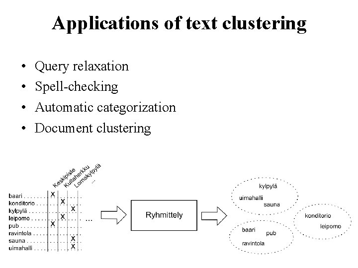
Applications of text clustering • • Query relaxation Spell-checking Automatic categorization Document clustering

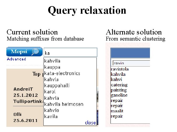
Query relaxation Current solution Matching suffixes from database Alternate solution From semantic clustering

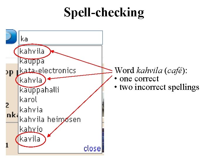
Spell-checking Word kahvila (café): • one correct • two incorrect spellings

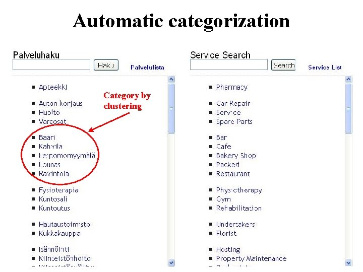
Automatic categorization Category by clustering

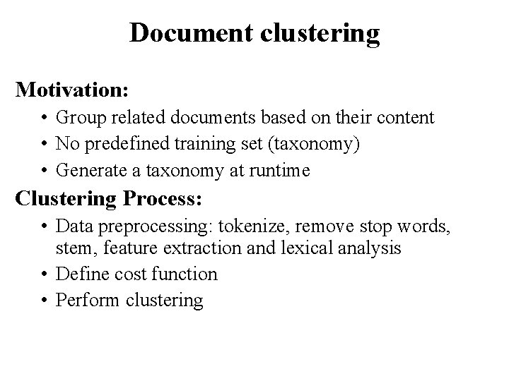
Document clustering Motivation: • Group related documents based on their content • No predefined training set (taxonomy) • Generate a taxonomy at runtime Clustering Process: • Data preprocessing: tokenize, remove stop words, stem, feature extraction and lexical analysis • Define cost function • Perform clustering

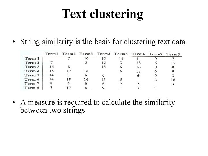
Text clustering • String similarity is the basis for clustering text data • A measure is required to calculate the similarity between two strings

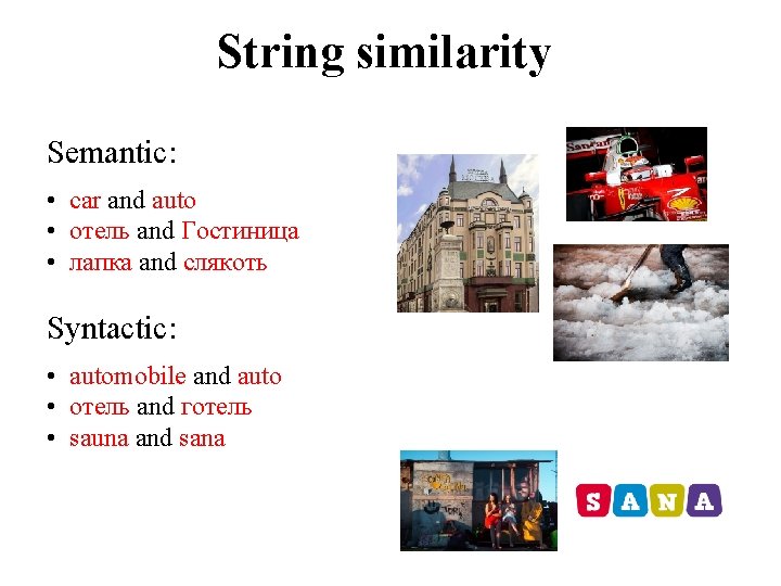
String similarity Semantic: • car and auto • отель and Гостиница • лапка and слякоть Syntactic: • automobile and auto • отель and готель • sauna and sana

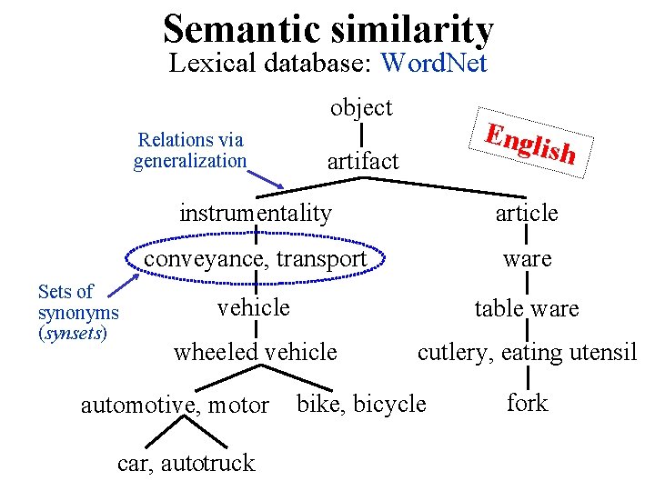
Semantic similarity Lexical database: Word. Net object Relations via generalization Sets of synonyms (synsets) Engl ish artifact instrumentality article conveyance, transport ware vehicle table ware wheeled vehicle cutlery, eating utensil automotive, motor car, autotruck bike, bicycle fork

Similarity using Word. Net [Wu and Palmer, 2004] Input : word 1: wolf , word 2: hunting dog Output: similarity value = 0. 89

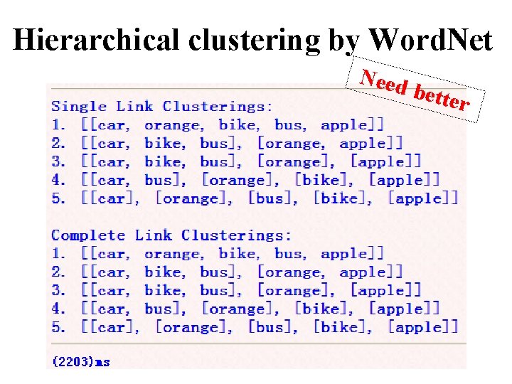
Hierarchical clustering by Word. Net Need bette r

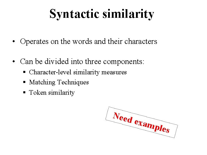
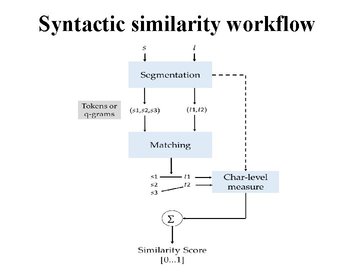
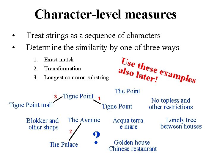
Syntactic similarity • Operates on the words and their characters • Can be divided into three components: § Character-level similarity measures § Matching Techniques § Token similarity Need exam ples

Syntactic similarity workflow

Character-level measures • • Treat strings as a sequence of characters Determine the similarity by one of three ways 1. 2. 3. Exact match Transformation Longest common substring 3 Tigne Point mall Blokker and other shops Tigne Point 1 Use t also l hese exa mple ater! s The Point Tigne Point The Avenue 2 The Palace ? No topless and other restrictions Acqua terra e mare Golden house Chinese restaurant Lonely tree between houses

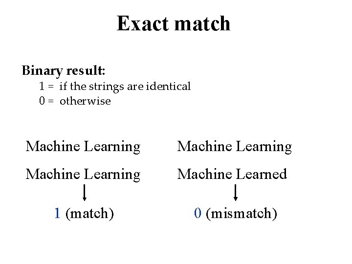
Exact match Binary result: 1 = if the strings are identical 0 = otherwise Machine Learning Machine Learned 1 (match) 0 (mismatch)

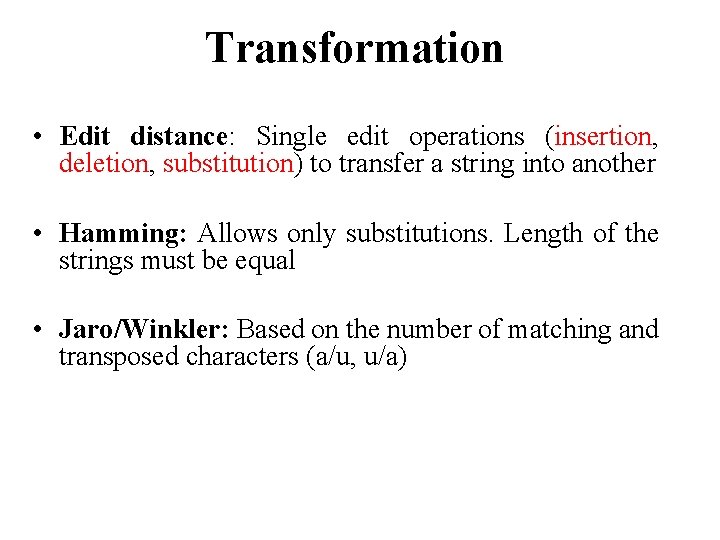
Transformation • Edit distance: Single edit operations (insertion, deletion, substitution) to transfer a string into another • Hamming: Allows only substitutions. Length of the strings must be equal • Jaro/Winkler: Based on the number of matching and transposed characters (a/u, u/a)

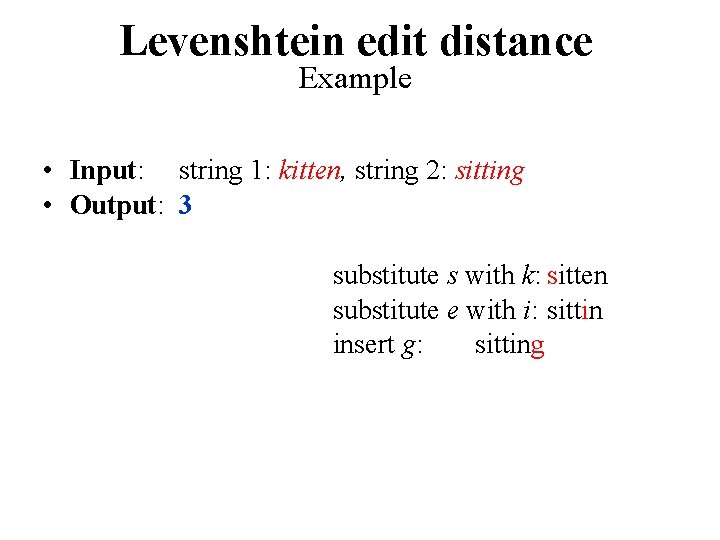
Levenshtein edit distance Example • Input: string 1: kitten, string 2: sitting • Output: 3 substitute s with k: sitten substitute e with i: sittin insert g: sitting

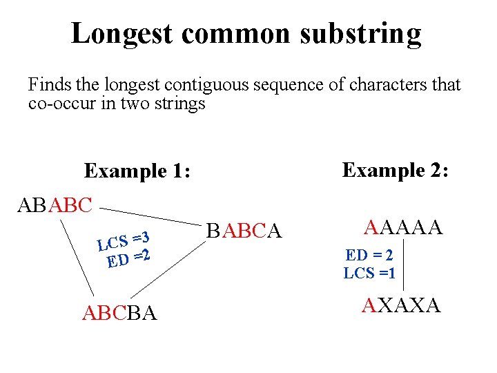
Longest common substring Finds the longest contiguous sequence of characters that co-occur in two strings Example 2: Example 1: ABABC 3 = S C L ED =2 ABCBA BABCA AAAAA ED = 2 LCS =1 AXAXA

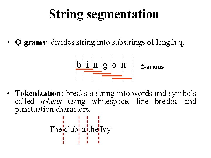
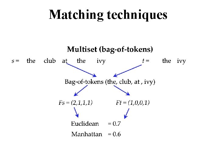
String segmentation • Q-grams: divides string into substrings of length q. b i n g o n 2 -grams • Tokenization: breaks a string into words and symbols called tokens using whitespace, line breaks, and punctuation characters. The club at the Ivy

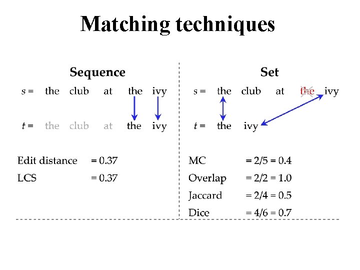
Matching techniques

Matching techniques

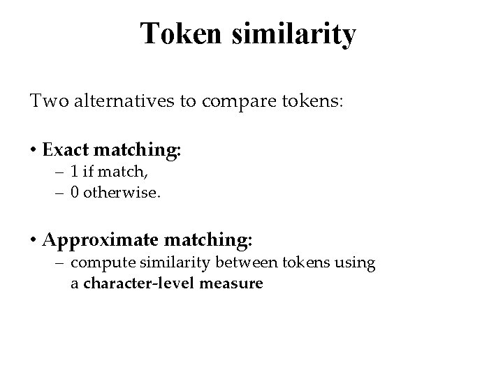
Token similarity Two alternatives to compare tokens: • Exact matching: – 1 if match, – 0 otherwise. • Approximate matching: – compute similarity between tokens using a character-level measure

Approximate matching Example [Monge and Elkan , 1996] Input: string 1: gray color, string 2: the grey colour Output: similarity value 0. 85 Pairwise similarities using edit distance (smith-waterman-Gotoh) the grey colour Maximum gray 0. 20 0. 90 0. 30 0. 90 color 0. 20 0. 30 0. 80

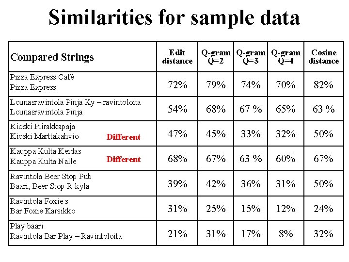
Similarities for sample data Edit Q-gram Cosine distance Q=2 Q=3 Q=4 distance Compared Strings Pizza Express Café Pizza Express 72% 79% 74% 70% 82% Lounasravintola Pinja Ky – ravintoloita Lounasravintola Pinja 54% 68% 67 % 65% 63 % Kioski Piirakkapaja Kioski Marttakahvio Different 47% 45% 33% 32% 50% Kauppa Kulta Keidas Kauppa Kulta Nalle Different 68% 67% 63 % 60% 67% Ravintola Beer Stop Pub Baari, Beer Stop R-kylä 39% 42% 36% 31% 50% Ravintola Foxie s Bar Foxie Karsikko 31% 25% 12% 24% Play baari Ravintola Bar Play – Ravintoloita 21% 31% 17% 8% 32%

Part V: Time series

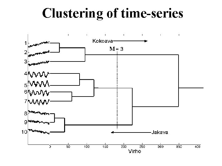
Clustering of time-series

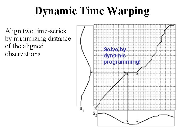
Dynamic Time Warping Align two time-series by minimizing distance of the aligned observations Solve by dynamic programming!

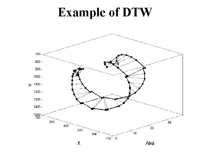
Example of DTW

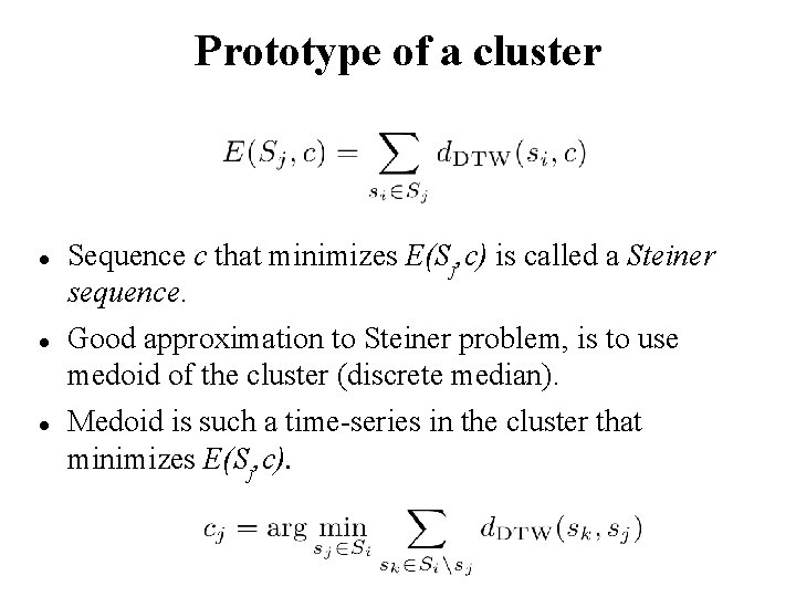
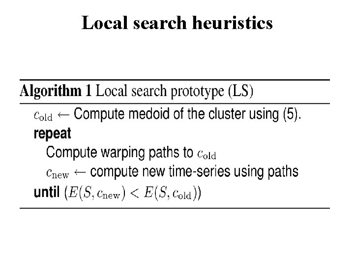
Prototype of a cluster Sequence c that minimizes E(Sj, c) is called a Steiner sequence. Good approximation to Steiner problem, is to use medoid of the cluster (discrete median). Medoid is such a time-series in the cluster that minimizes E(Sj, c).

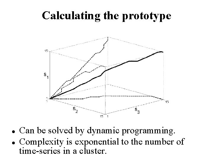
Calculating the prototype Can be solved by dynamic programming. Complexity is exponential to the number of time-series in a cluster.

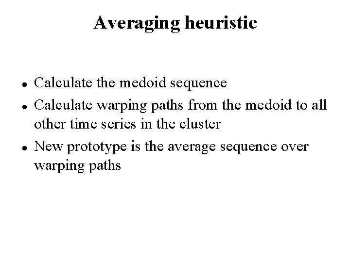
Averaging heuristic Calculate the medoid sequence Calculate warping paths from the medoid to all other time series in the cluster New prototype is the average sequence over warping paths

Local search heuristics

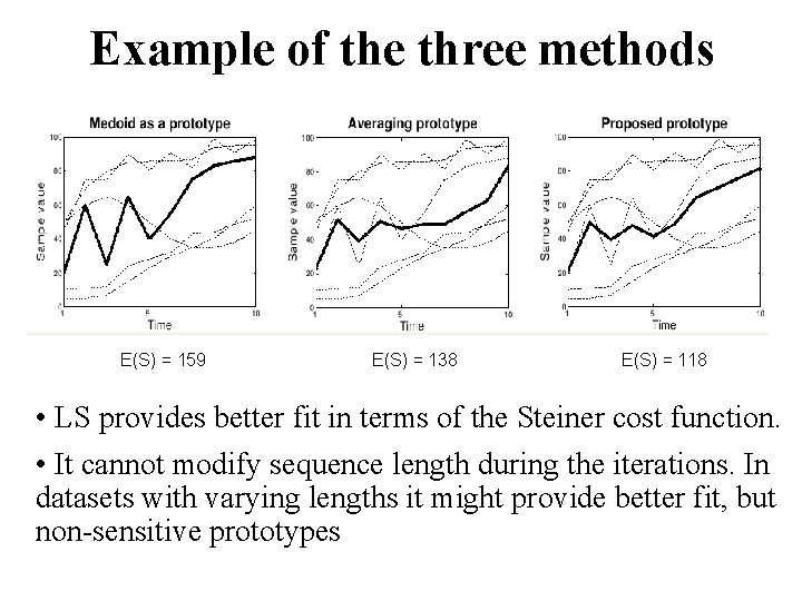
Example of the three methods E(S) = 159 E(S) = 138 E(S) = 118 • LS provides better fit in terms of the Steiner cost function. • It cannot modify sequence length during the iterations. In datasets with varying lengths it might provide better fit, but non-sensitive prototypes

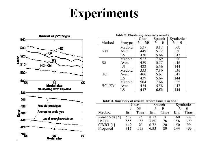
Experiments

Part VI: Other clustering problems

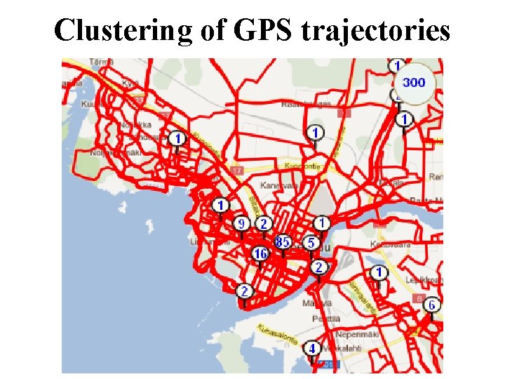
Clustering of GPS trajectories

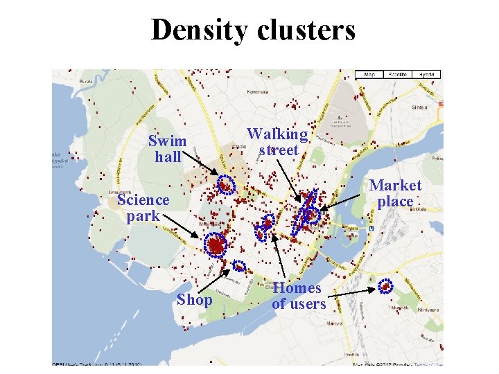
Density clusters Swim hall Walking street Market place Science park Shop Homes of users

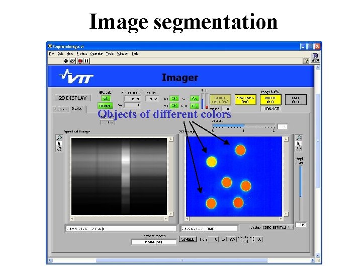
Image segmentation Objects of different colors

Literature 1. S. Theodoridis and K. Koutroumbas, Pattern Recognition, Academic Press, 2 nd edition, 2006. 2. P. Fränti and T. Kaukoranta, "Binary vector quantizer design using soft centroids", Signal Processing: Image Communication, 14 (9), 677‑ 681, 1999. 3. I. Kärkkäinen and P. Fränti, "Variable metric for binary vector quantization", IEEE Int. Conf. on Image Processing (ICIP’ 04), Singapore, vol. 3, 3499 -3502, October 2004. 4. Michael Pucher, F. T. W. : Performance Evaluation of Word. Net-based Semantic Relatedness Measures for Word Prediction in Conversational Speech (2004) 5. A. E. Monge, and C. Elkan. The Field Matching Problem: Algorithms and Applications. Int. Conf. on Knowledge Discovery and Data Mining, 267 -270, 1996.