Clustering Basic Concepts and Algorithms Bamshad Mobasher De

Clustering Basic Concepts and Algorithms Bamshad Mobasher De. Paul University

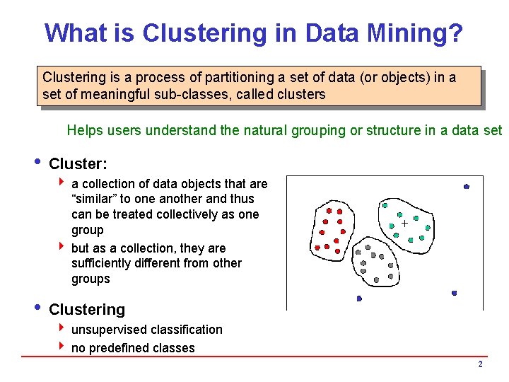
What is Clustering in Data Mining? Clustering is a process of partitioning a set of data (or objects) in a set of meaningful sub-classes, called clusters Helps users understand the natural grouping or structure in a data set i Cluster: 4 a collection of data objects that are “similar” to one another and thus can be treated collectively as one group 4 but as a collection, they are sufficiently different from other groups i Clustering 4 unsupervised classification 4 no predefined classes 2

Applications of Cluster Analysis i Data reduction 4 Summarization: Preprocessing for regression, PCA, classification, and association analysis 4 Compression: Image processing: vector quantization i Hypothesis generation and testing i Prediction based on groups 4 Cluster & find characteristics/patterns for each group i Finding K-nearest Neighbors 4 Localizing search to one or a small number of clusters i Outlier detection: Outliers are often viewed as those “far away” from any cluster 3

Basic Steps to Develop a Clustering Task i Feature selection / Preprocessing 4 Select info concerning the task of interest 4 Minimal information redundancy 4 May need to do normalization/standardization i Distance/Similarity measure 4 Similarity of two feature vectors i Clustering criterion 4 Expressed via a cost function or some rules i Clustering algorithms 4 Choice of algorithms i Validation of the results i Interpretation of the results with applications 4

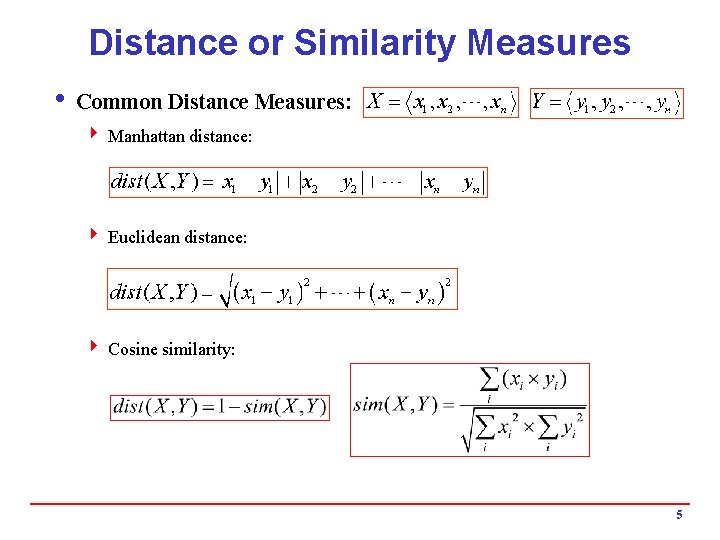
Distance or Similarity Measures i Common Distance Measures: 4 Manhattan distance: 4 Euclidean distance: 4 Cosine similarity: 5

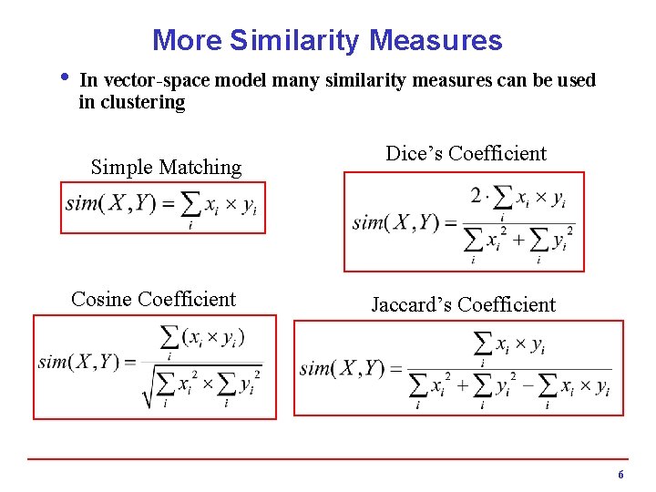
More Similarity Measures i In vector-space model many similarity measures can be used in clustering Simple Matching Cosine Coefficient Dice’s Coefficient Jaccard’s Coefficient 6

Quality: What Is Good Clustering? i A good clustering method will produce high quality clusters 4 high intra-class similarity: cohesive within clusters 4 low inter-class similarity: distinctive between clusters i The quality of a clustering method depends on 4 the similarity measure used 4 its implementation, and 4 Its ability to discover some or all of the hidden patterns 7

Major Clustering Approaches i Partitioning approach: 4 Construct various partitions and then evaluate them by some criterion, e. g. , minimizing the sum of square errors 4 Typical methods: k-means, k-medoids, CLARANS i Hierarchical approach: 4 Create a hierarchical decomposition of the set of data (or objects) using some criterion 4 Typical methods: Diana, Agnes, BIRCH, CAMELEON i Density-based approach: 4 Based on connectivity and density functions 4 Typical methods: DBSCAN, OPTICS, Den. Clue i Model-based: 4 A model is hypothesized for each of the clusters and tries to find the best fit of that model to each other 4 Typical methods: EM, SOM, COBWEB 8

Partitioning Approaches i The notion of comparing item similarities can be extended to clusters themselves, by focusing on a representative vector for each cluster 4 cluster representatives can be actual items in the cluster or other “virtual” representatives such as the centroid 4 this methodology reduces the number of similarity computations in clustering 4 clusters are revised successively until a stopping condition is satisfied, or until no more changes to clusters can be made i Reallocation-Based Partitioning Methods 4 Start with an initial assignment of items to clusters and then move items from cluster to obtain an improved partitioning 4 Most common algorithm: k-means 9

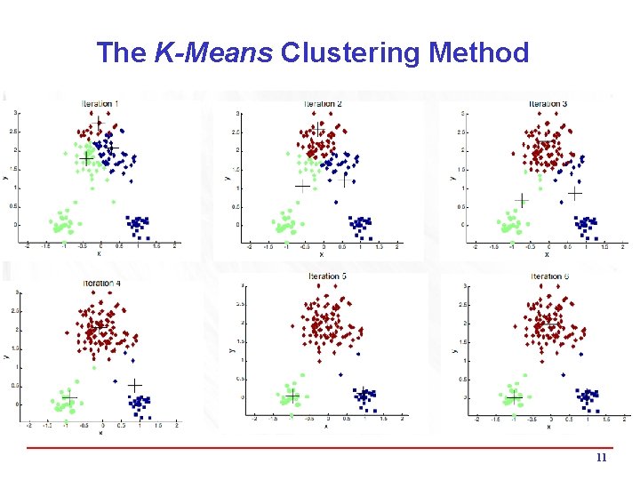
The K-Means Clustering Method i Given the number of desired clusters k, the k-means algorithm follows four steps: 1. Randomly assign objects to create k nonempty initial partitions (clusters) 2. Compute the centroids of the clusters of the current partitioning (the centroid is the center, i. e. , mean point, of the cluster) 3. Assign each object to the cluster with the nearest centroid (reallocation step) 4. Go back to Step 2, stop when the assignment does not change 10

The K-Means Clustering Method 11

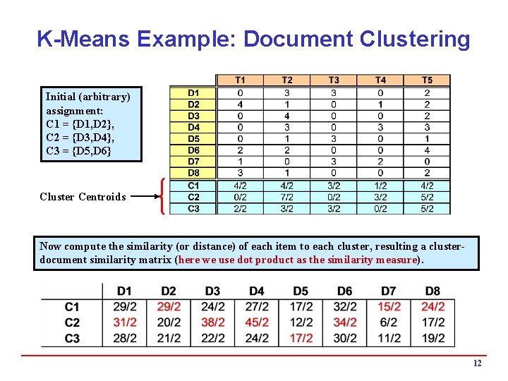
K-Means Example: Document Clustering Initial (arbitrary) assignment: C 1 = {D 1, D 2}, C 2 = {D 3, D 4}, C 3 = {D 5, D 6} Cluster Centroids Now compute the similarity (or distance) of each item to each cluster, resulting a clusterdocument similarity matrix (here we use dot product as the similarity measure). 12

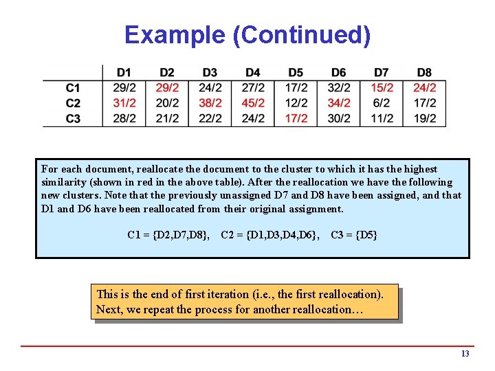
Example (Continued) For each document, reallocate the document to the cluster to which it has the highest similarity (shown in red in the above table). After the reallocation we have the following new clusters. Note that the previously unassigned D 7 and D 8 have been assigned, and that D 1 and D 6 have been reallocated from their original assignment. C 1 = {D 2, D 7, D 8}, C 2 = {D 1, D 3, D 4, D 6}, C 3 = {D 5} This is the end of first iteration (i. e. , the first reallocation). Next, we repeat the process for another reallocation… 13

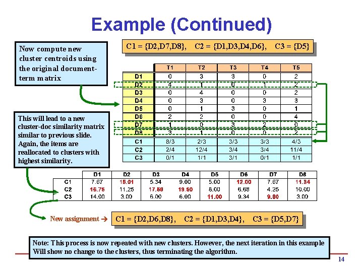
Example (Continued) Now compute new cluster centroids using the original documentterm matrix C 1 = {D 2, D 7, D 8}, C 2 = {D 1, D 3, D 4, D 6}, C 3 = {D 5} This will lead to a new cluster-doc similarity matrix similar to previous slide. Again, the items are reallocated to clusters with highest similarity. New assignment C 1 = {D 2, D 6, D 8}, C 2 = {D 1, D 3, D 4}, C 3 = {D 5, D 7} Note: This process is now repeated with new clusters. However, the next iteration in this example Will show no change to the clusters, thus terminating the algorithm. 14

K-Means Algorithm i Strength of the k-means: 4 Relatively efficient: O(tkn), where n is # of objects, k is # of clusters, and t is # of iterations. Normally, k, t << n 4 Often terminates at a local optimum i Weakness of the k-means: 4 Applicable only when mean is defined; what about categorical data? 4 Need to specify k, the number of clusters, in advance 4 Unable to handle noisy data and outliers i Variations of K-Means usually differ in: 4 Selection of the initial k means 4 Distance or similarity measures used 4 Strategies to calculate cluster means 15

A Disk Version of k-means i k-means can be implemented with data on disk 4 In each iteration, it scans the database once 4 The centroids are computed incrementally i It can be used to cluster large datasets that do not fit in main memory i We need to control the number of iterations 4 In practice, a limited is set (< 50) i There are better algorithms that scale up for large data sets, e. g. , BIRCH 16

BIRCH i. Designed for very large data sets 4 Time and memory are limited 4 Incremental and dynamic clustering of incoming objects 4 Only one scan of data is necessary 4 Does not need the whole data set in advance i. Two key phases: 4 Scans the database to build an in-memory tree 4 Applies clustering algorithm to cluster the leaf nodes 17

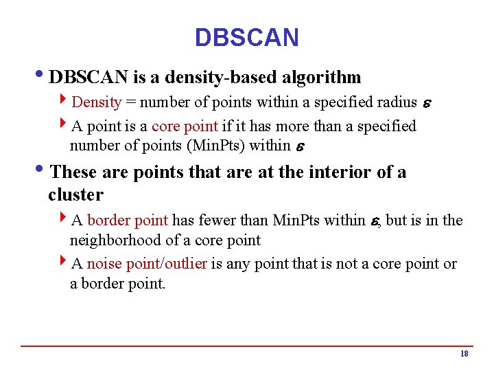
DBSCAN is a density-based algorithm 4 Density = number of points within a specified radius 4 A point is a core point if it has more than a specified number of points (Min. Pts) within i. These are points that are at the interior of a cluster 4 A border point has fewer than Min. Pts within , but is in the neighborhood of a core point 4 A noise point/outlier is any point that is not a core point or a border point. 18

DBSCAN i. Two parameters: 4ε: Maximum radius of the neighborhood 4 Min. Pts: Minimum number of points in an ε-neighborhood of a given point p 4 Nε (p): {q belongs to D | dist(p, q) <= ε} i. Directly density-reachable: A point q is directly density-reachable from a point p wrt. ε, Min. Pts if: 41) q belongs to Nε (p): 42) core point condition: | Nε (p) | >= Min. Pts 19

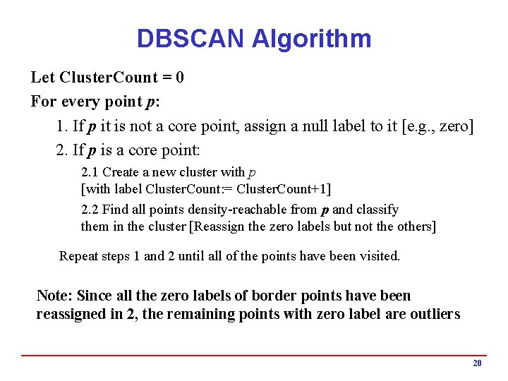
DBSCAN Algorithm Let Cluster. Count = 0 For every point p: 1. If p it is not a core point, assign a null label to it [e. g. , zero] 2. If p is a core point: 2. 1 Create a new cluster with p [with label Cluster. Count: = Cluster. Count+1] 2. 2 Find all points density-reachable from p and classify them in the cluster [Reassign the zero labels but not the others] Repeat steps 1 and 2 until all of the points have been visited. Note: Since all the zero labels of border points have been reassigned in 2, the remaining points with zero label are outliers 20

DBSCAN i. Advantage: 4 Can find clusters of arbitrary shape (whereas K-Means can only find spherical shaped clusters 4 Good at handling noise and finding outliers i. Disadvantages: 4 Needs to parameters ε, and Min. Pts 4 The optimal values of ε could be difficult to determine 21

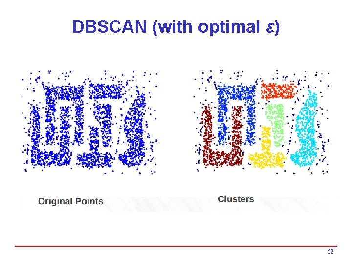
DBSCAN (with optimal ε) 22

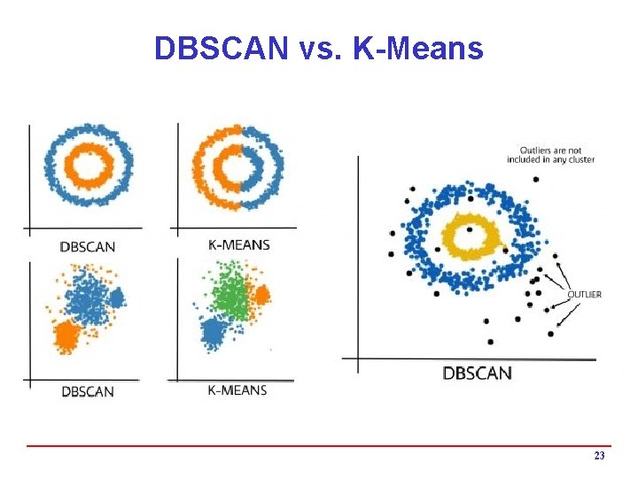
DBSCAN vs. K-Means 23

Hierarchical Clustering Algorithms • Two main types of hierarchical clustering – Agglomerative: • Start with the points as individual clusters • At each step, merge the closest pair of clusters until only one cluster (or k clusters) left – Divisive: • Start with one, all-inclusive cluster • At each step, split a cluster until each cluster contains a point (or there are k clusters) • Traditional hierarchical algorithms use a similarity or distance matrix – Merge or split one cluster at a time

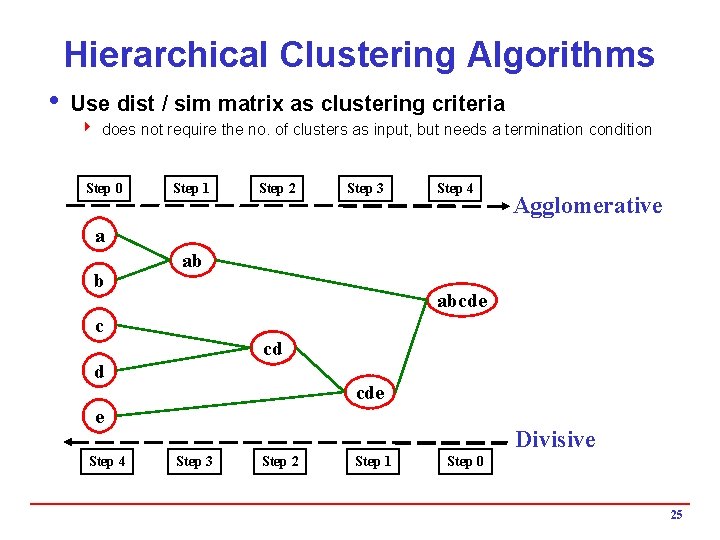
Hierarchical Clustering Algorithms i Use dist / sim matrix as clustering criteria 4 does not require the no. of clusters as input, but needs a termination condition Step 0 Step 1 Step 2 Step 3 Step 4 Agglomerative a b ab abcde c cd d cde e Step 4 Divisive Step 3 Step 2 Step 1 Step 0 25

Hierarchical Agglomerative Clustering i. Basic procedure 41. Place each of N items into a cluster of its own. 42. Compute all pairwise item-item similarity coefficients h. Total of N(N-1)/2 coefficients 43. Form a new cluster by combining the most similar pair of current clusters i and j h(methods for determining which clusters to merge: single-link, complete link, group average, etc. ); hupdate similarity matrix by deleting the rows and columns corresponding to i and j; hcalculate the entries in the row corresponding to the new cluster i+j. 44. Repeat step 3 if the number of clusters left is great than 1. 26

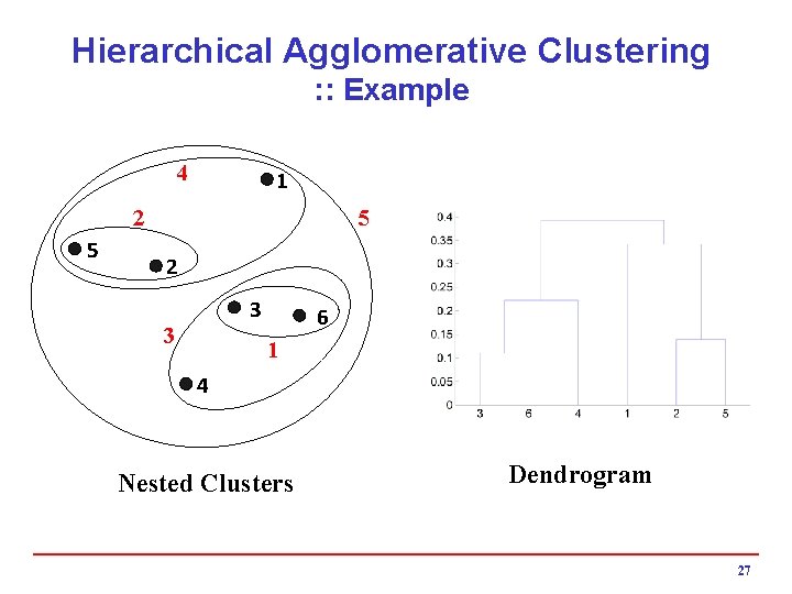
Hierarchical Agglomerative Clustering : : Example 4 1 5 2 3 3 6 1 4 Nested Clusters Dendrogram 27

Distance Between Two Clusters i The basic procedure varies based on the method used to determine inter-cluster distances or similarities i Different methods results in different variants of the algorithm 4 Single link 4 Complete link 4 Average link 4 Ward’s method 4 Etc. 28

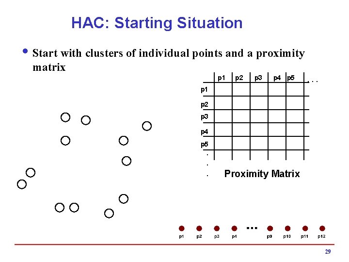
HAC: Starting Situation i Start with clusters of individual points and a proximity matrix p 1 p 2 p 3 p 4 p 5 . . . p 1 p 2 p 3 p 4 p 5. . . Proximity Matrix 29

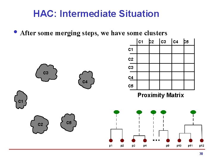
HAC: Intermediate Situation i After some merging steps, we have some clusters C 1 C 2 C 3 C 4 C 5 Proximity Matrix C 1 C 2 C 5 30

HAC: Join Step i We want to merge the two closest clusters (C 2 and C 5) and update the proximity matrix. C 1 C 2 C 3 C 4 C 5 C 1 C 2 C 3 C 4 C 3 C 5 C 4 Proximity Matrix C 1 C 2 C 5 31

After Merging i The question is “How do we update the proximity matrix? ” C 1 C 2 U C 5 C 3 C 4 ? ? ? C 3 ? C 4 ? Proximity Matrix C 1 C 2 U C 5 32

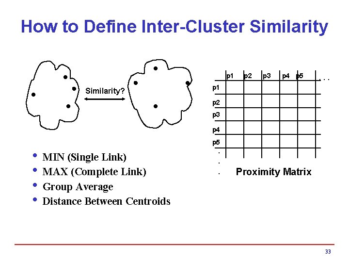
How to Define Inter-Cluster Similarity p 1 Similarity? p 2 p 3 p 4 p 5 . . . p 1 p 2 p 3 p 4 p 5 i MIN (Single Link) i MAX (Complete Link) i Group Average i Distance Between Centroids . . . Proximity Matrix 33

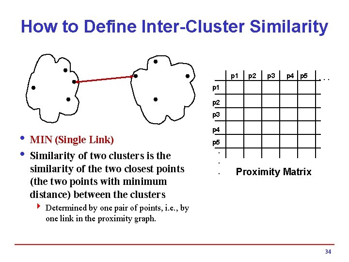
How to Define Inter-Cluster Similarity p 1 p 2 p 3 p 4 p 5 . . . p 1 p 2 p 3 i MIN (Single Link) i Similarity of two clusters is the similarity of the two closest points (the two points with minimum distance) between the clusters p 4 p 5. . . Proximity Matrix 4 Determined by one pair of points, i. e. , by one link in the proximity graph. 34

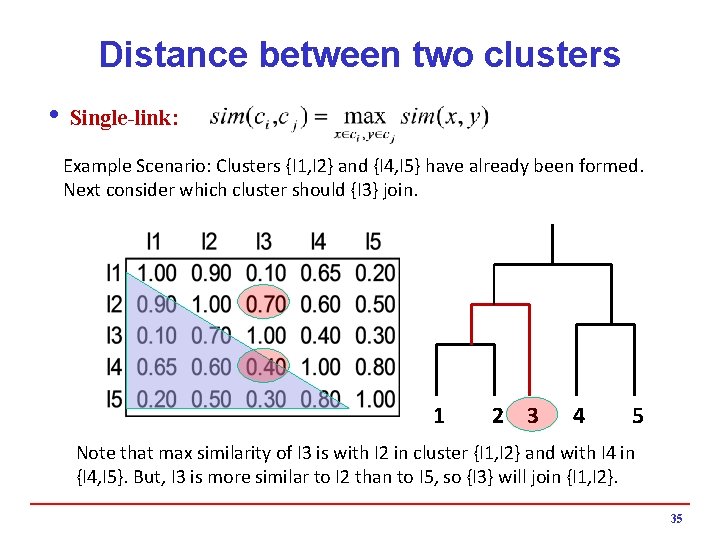
Distance between two clusters i Single-link: Example Scenario: Clusters {I 1, I 2} and {I 4, I 5} have already been formed. Next consider which cluster should {I 3} join. 1 2 3 4 5 Note that max similarity of I 3 is with I 2 in cluster {I 1, I 2} and with I 4 in {I 4, I 5}. But, I 3 is more similar to I 2 than to I 5, so {I 3} will join {I 1, I 2}. 35

How to Define Inter-Cluster Similarity p 1 p 2 p 3 p 4 p 5 . . . p 1 p 2 p 3 i Max (Complete Link) i Similarity of two clusters is based on the similarity of the two least similar (most distant) points between the clusters p 4 p 5. . . Proximity Matrix 36

Distance between two clusters i Complete Link: Example: Clusters {I 1, I 2} and {I 4, I 5} have already been formed. Again, let’s consider whether {3} should be joined with {I 1, I 2} or with {I 4, I 5}. 1 2 3 4 5 Note that min similarity of I 3 is with I 5 in {I 4, I 5} and with I 1 in {I 1, I 2}. But, I 3 is more similar to I 5 than to I 1. 37

How to Define Inter-Cluster Similarity p 1 p 2 p 3 p 4 p 5 . . . p 1 p 2 p 3 i Group Average i Similarity of two clusters is the average of pairwise similarity between points in the two clusters p 4 p 5. . . Proximity Matrix 38

Distance between two clusters i Group average: 1 2 3 4 5 39

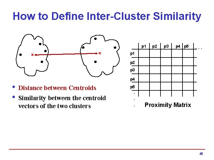
How to Define Inter-Cluster Similarity p 1 p 2 p 3 p 4 p 5 . . . p 1 p 2 p 3 p 4 i Distance between Centroids i Similarity between the centroid vectors of the two clusters p 5. . . Proximity Matrix 40

Measures of Cluster Quality i. Numerical measures that are applied to judge various aspects of cluster quality: 4 External Criteria: Used to measure the extent to which cluster labels match externally supplied class labels. hentropy, completeness/homogeneity. 4 Internal Criteria: Used to measure the goodness of a clustering structure without respect to external information. h. Sum of Squared Error (SSE) h. Cohesion/Separation 4 Relative Criteria: Used to compare two different clusterings or clusters. 41

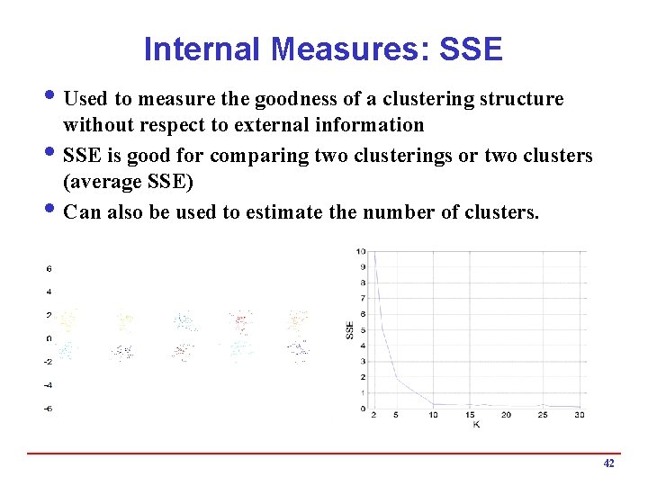
Internal Measures: SSE i Used to measure the goodness of a clustering structure without respect to external information i SSE is good for comparing two clusterings or two clusters (average SSE) i Can also be used to estimate the number of clusters. 42

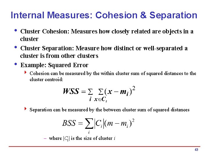
Internal Measures: Cohesion & Separation i Cluster Cohesion: Measures how closely related are objects in a cluster i Cluster Separation: Measure how distinct or well-separated a cluster is from other clusters i Example: Squared Error 4 Cohesion can be measured by the within cluster sum of squared distances to the cluster centroid: 4 Separation can be measured by the between cluster sum of squared distances – where |Ci| is the size of cluster i 43

Internal Measures: Cohesion & Separation i A proximity graph based approach can also be used for cohesion and separation. 4 Cluster cohesion is the sum of the weight of all links within a cluster. 4 Cluster separation is the sum of the weights between nodes in the cluster and nodes outside the cluster. cohesion separation

Internal Measures: Silhouette Coefficient i Silhouette Coefficient combines cohesion and separation, but for individual points, as well as clusters i For an individual point, i 4 Calculate a(i) = average distance of i to the points in its cluster 4 Calculate b(i) = min (average distance of i to points in another cluster) 4 The silhouette coefficient for a point is then given by: 4 Typically between 0 and 1 4 The closer to 1 the better i Can calculate the Average Silhouette width for a clustering 45