Clustering 1 Types of Data Partitioning methods Hierarchical

Clustering 1

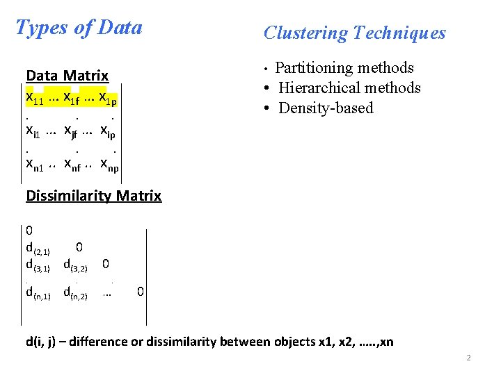
Types of Data Partitioning methods • Hierarchical methods • Density-based • Data Matrix x 11 … x 1 f … x 1 p. . . Clustering Techniques xi 1 … xjf … xip xn 1. . xnf. . xnp Dissimilarity Matrix 0 d(2, 1) 0 d(3, 1) d(3, 2). . d(n, 1) d(n, 2) 0. … 0 d(i, j) – difference or dissimilarity between objects x 1, x 2, …. . , xn 2

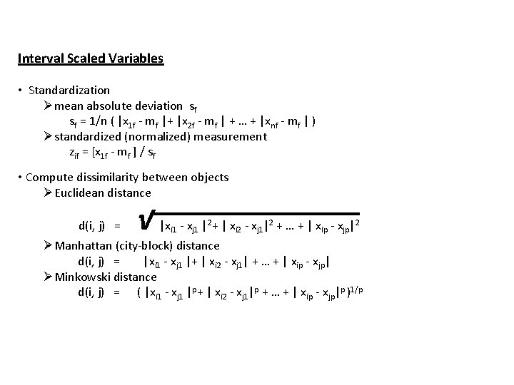
Interval Scaled Variables • Standardization Ømean absolute deviation sf sf = 1/n ( |x 1 f - mf |+ |x 2 f - mf | + … + |xnf - mf | ) Østandardized (normalized) measurement zif = [x 1 f - mf ] / sf • Compute dissimilarity between objects ØEuclidean distance d(i, j) = √ |x - x | + | x - x | + … + | x - x | i 1 j 1 2 i 2 j 1 2 ip jp 2 ØManhattan (city-block) distance d(i, j) = |xi 1 - xj 1 |+ | xi 2 - xj 1| + … + | xip - xjp| ØMinkowski distance d(i, j) = ( |xi 1 - xj 1 |p+ | xi 2 - xj 1|p + … + | xip - xjp|p )1/p

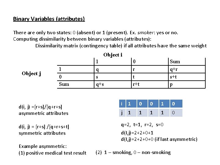
Binary Variables (attributes) There are only two states: 0 (absent) or 1 (present). Ex. smoker: yes or no. Computing dissimilarity between binary variables (attributes): Dissimilarity matrix (contingency table) if all attributes have the same weight Object i Object j 1 0 Sum d(i, j) =[r+s]/[q+r+s] asymmetric attributes d(i, j) = [r+s] /[q+r+s+t] symmetric attributes Example asymmetric: (1) positive medical test result 1 q s q+s 0 r t r+t Sum q+r s+t p i 1 0 0 1 0 j 1 1 0 q=2, t=1, r=2, s=0 d(I, j)=2+2+0+1 d(I, j)=2+2+0+0 (if last asymmetric) (2) 1 – smoking, 0 – non-smoking

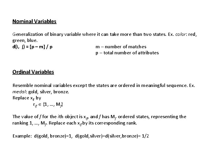
Nominal Variables Generalization of binary variable where it can take more than two states. Ex. color: red, green, blue. d(i, j) = [p – m] / p m – number of matches p – total number of attributes Ordinal Variables Resemble nominal variables except the states are ordered in meaningful sequence. Ex. medal: gold, silver, bronze. Replace xif by rif {1, …, Mf} The value of f for the ith object is xif, and f has Mf ordered states, representing the ranking 1, …, Mf. Replace each xif by its corresponding rank. Example: d(gold, bronze)=1, d(gold, silver)=d(silver, bronze)= 1/2

Hierarchical Attribute a[1] 1/2 a[11] 1/4 a[111] 1/8 a[1111] a 1 a[2] a[12] a[21] a[112] a[1121] a[1] can be either a[11] or a[12] d(a[111], a[1121])=1/4, d(a[1], a[11])= [d(a[11], a[11])+d(a[11], a[12])]/2= [½ + ¼]/2=3/8

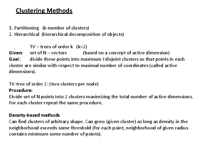
Clustering Methods 1. Partitioning (k-number of clusters) 2. Hierarchical (hierarchical decomposition of objects) TV – trees of order k (k=2) Given: set of N – vectors (based on a concept of active dimension) Goal: divide these points into maximum I disjoint clusters so that points in each cluster are similar with respect to maximal number of coordinates (called active dimensions). TV-tree of order 2: (two clusters per node) Procedure: Divide set of N points into 2 clusters maximizing the total number of active dimensions. For each cluster repeat the same procedure. Density-based methods Can find clusters of arbitrary shape. Can grow (given cluster) as long as density in the neighborhood exceeds some threshold (for each point, neighborhood of given radius contains minimum some number of points).

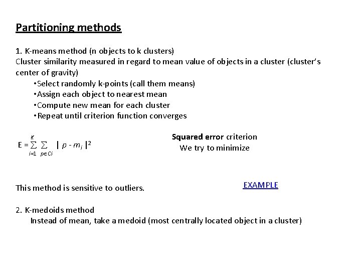
Partitioning methods 1. K-means method (n objects to k clusters) Cluster similarity measured in regard to mean value of objects in a cluster (cluster’s center of gravity) • Select randomly k-points (call them means) • Assign each object to nearest mean • Compute new mean for each cluster • Repeat until criterion function converges K E = | p - mi |2 i=1 p Ci This method is sensitive to outliers. Squared error criterion We try to minimize EXAMPLE 2. K-medoids method Instead of mean, take a medoid (most centrally located object in a cluster)

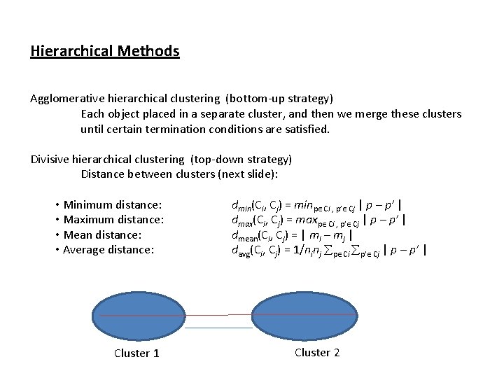
Hierarchical Methods Agglomerative hierarchical clustering (bottom-up strategy) Each object placed in a separate cluster, and then we merge these clusters until certain termination conditions are satisfied. Divisive hierarchical clustering (top-down strategy) Distance between clusters (next slide): • Minimum distance: • Maximum distance: • Mean distance: • Average distance: Cluster 1 dmin(Ci, Cj) = minp Ci , p’ Cj | p – p’ | dmax(Ci, Cj) = maxp Ci , p’ Cj | p – p’ | dmean(Ci, Cj) = | mi – mj | davg(Ci, Cj) = 1/ninj p Ci p’ Cj | p – p’ | Cluster 2

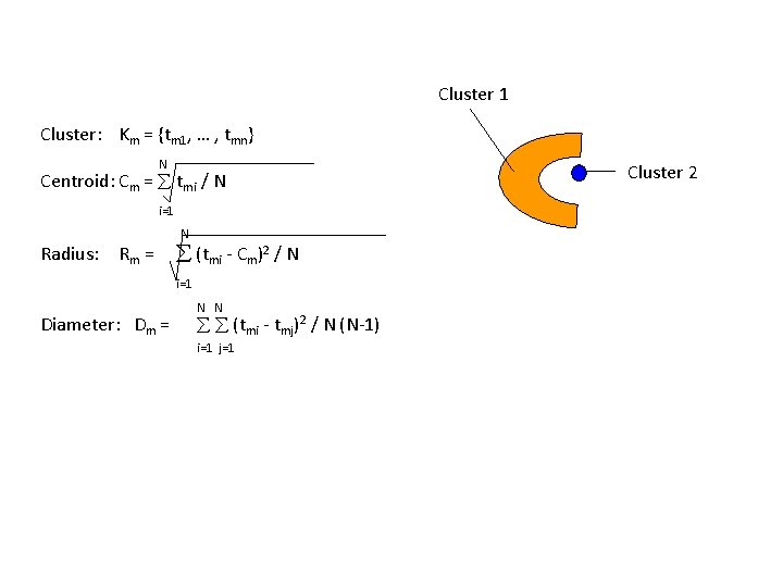
Cluster 1 Cluster: Km = {tm 1, … , tmn} N Centroid: Cm = tmi / N i=1 Radius: Rm = N (tmi - Cm)2 / N i=1 Diameter: Dm = N N (tmi - tmj)2 / N (N-1) i=1 j=1 Cluster 2

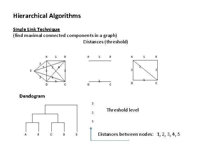
Hierarchical Algorithms Single Link Technique (find maximal connected components in a graph) Distances (threshold) A 3 E 3 2 3 1 2 5 D B 4 1 A 1 B A 2 2 C 1 D C D 1 2 B 2 1 C Dendogram 3 2 Threshold level 1 A B C D E Distances between nodes: 1, 2, 3, 4, 5

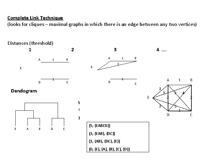
Complete Link Technique (looks for cliques – maximal graphs in which there is an edge between any two vertices) Distances (threshold) 1 A 2 1 3 A B 1 1 D C 1 Dendogram 5 3 1 E A B D C B 3 E E D 4 …. (5, {EABCD}) (3, {EAB}, {DC}) (1, {AB}, {DC}, {E}) (0, {E}, {A}, {B}, {C}, {D}) C

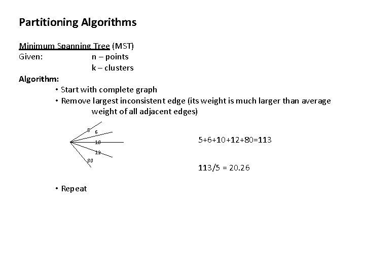
Partitioning Algorithms Minimum Spanning Tree (MST) Given: n – points k – clusters Algorithm: • Start with complete graph • Remove largest inconsistent edge (its weight is much larger than average weight of all adjacent edges) 5 6 10 5+6+10+12+80=113 12 80 • Repeat 113/5 = 20. 26

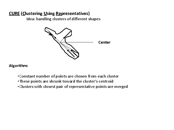
CURE (Clustering Using Representatives) Idea: handling clusters of different shapes Center Algorithm: • Constant number of points are chosen from each cluster • These points are shrunk toward the cluster’s centroid • Clusters with closest pair of representative points are merged