Cluster Analysis What is Cluster Analysis Types of

Cluster Analysis • What is Cluster Analysis? • Types of Data in Cluster Analysis • A Categorization of Major Clustering Methods • Partitioning Methods • Hierarchical Methods • Density-Based Methods • Grid-Based Methods • Model-Based Clustering Methods • Outlier Analysis • Summary

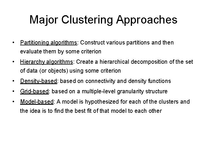
Major Clustering Approaches • Partitioning algorithms: Construct various partitions and then evaluate them by some criterion • Hierarchy algorithms: Create a hierarchical decomposition of the set of data (or objects) using some criterion • Density-based: based on connectivity and density functions • Grid-based: based on a multiple-level granularity structure • Model-based: A model is hypothesized for each of the clusters and the idea is to find the best fit of that model to each other

Cluster Analysis • What is Cluster Analysis? • Types of Data in Cluster Analysis • A Categorization of Major Clustering Methods • Partitioning Methods • Hierarchical Methods • Density-Based Methods • Grid-Based Methods • Model-Based Clustering Methods • Outlier Analysis • Summary

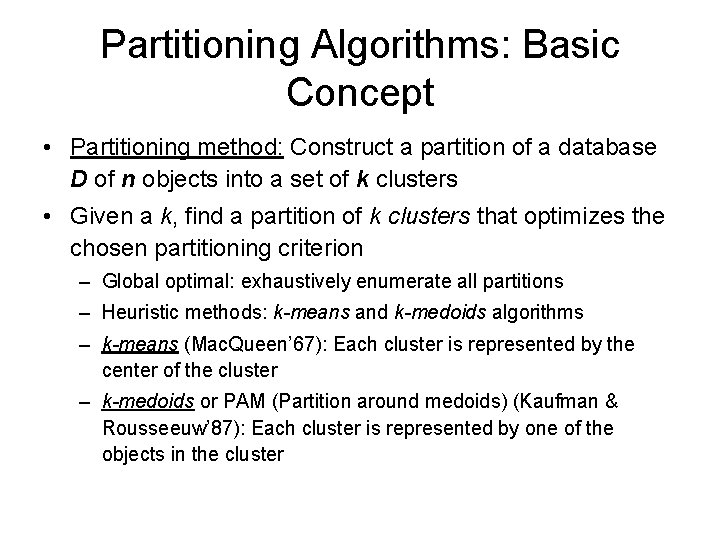
Partitioning Algorithms: Basic Concept • Partitioning method: Construct a partition of a database D of n objects into a set of k clusters • Given a k, find a partition of k clusters that optimizes the chosen partitioning criterion – Global optimal: exhaustively enumerate all partitions – Heuristic methods: k-means and k-medoids algorithms – k-means (Mac. Queen’ 67): Each cluster is represented by the center of the cluster – k-medoids or PAM (Partition around medoids) (Kaufman & Rousseeuw’ 87): Each cluster is represented by one of the objects in the cluster

The K-Means Clustering Method • Given k, the k-means algorithm is implemented in four steps: – Partition objects into k nonempty subsets – Compute seed points as the centroids of the clusters of the current partition (the centroid is the center, i. e. , mean point, of the cluster) – Assign each object to the cluster with the nearest seed point – Go back to Step 2, stop when no more new assignment

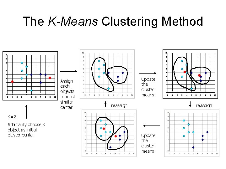
The K-Means Clustering Method 10 10 9 9 8 8 7 7 6 6 5 5 4 3 2 1 0 0 1 2 3 4 5 6 7 8 9 10 Assign each objects to most similar center Update the cluster means reassign 3 2 1 0 0 1 2 3 4 5 6 7 8 9 reassign K=2 Arbitrarily choose K object as initial cluster center 4 Update the cluster means 10

Comments on the K-Means Method • Strength: Relatively efficient: O(tkn), where n is # objects, k is # clusters, and t is # iterations. Normally, k, t << n. • Comparing: PAM: O(k(n-k)2 ), CLARA: O(ks 2 + k(n-k)) • Comment: Often terminates at a local optimum. [Ignore the comment in book: the global optimum may be found using techniques such as: deterministic annealing and genetic algorithms] • Weakness – Applicable only when mean is defined, then what about categorical data? – Need to specify k, the number of clusters, in advance – Unable to handle noisy data and outliers – Not suitable to discover clusters with non-convex shapes

Variations of the K-Means Method • A few variants of the k-means which differ in – Selection of the initial k means – Dissimilarity calculations – Strategies to calculate cluster means • Handling categorical data: k-modes (Huang’ 98) – Replacing means of clusters with modes – Using new dissimilarity measures to deal with categorical objects – Using a frequency-based method to update modes of clusters – A mixture of categorical and numerical data: k-prototype method

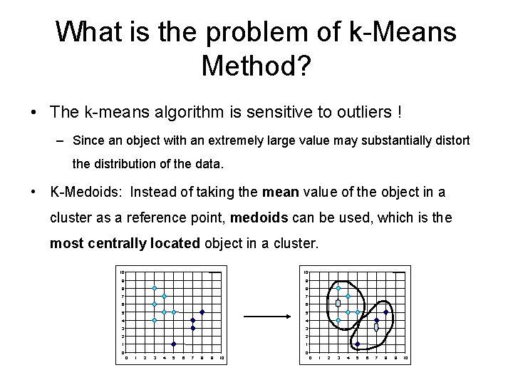
What is the problem of k-Means Method? • The k-means algorithm is sensitive to outliers ! – Since an object with an extremely large value may substantially distort the distribution of the data. • K-Medoids: Instead of taking the mean value of the object in a cluster as a reference point, medoids can be used, which is the most centrally located object in a cluster. 10 10 9 9 8 8 7 7 6 6 5 5 4 4 3 3 2 2 1 1 0 0 0 1 2 3 4 5 6 7 8 9 10

The K-Medoids Clustering Method • Find representative objects, called medoids, in clusters • PAM (Partitioning Around Medoids, 1987) – starts from an initial set of medoids and iteratively replaces one of the medoids by one of the non-medoids if it improves the total distance of the resulting clustering – PAM works effectively for small data sets, but does not scale well for large data sets • CLARA (Kaufmann & Rousseeuw, 1990) • CLARANS (Ng & Han, 1994): Randomized sampling • Focusing + spatial data structure (Ester et al. , 1995)

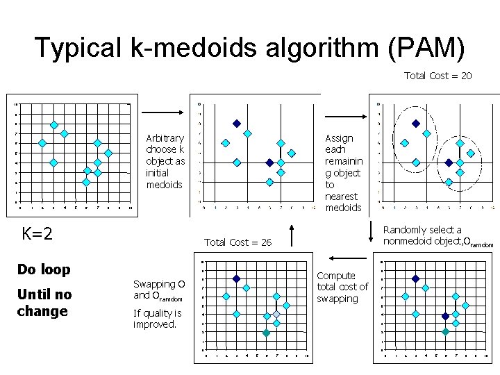
Typical k-medoids algorithm (PAM) Total Cost = 20 10 9 8 Arbitrary choose k object as initial medoids 7 6 5 4 3 2 Assign each remainin g object to nearest medoids 1 0 0 1 2 3 4 5 6 7 8 9 10 K=2 Do loop Until no change Randomly select a nonmedoid object, Oramdom Total Cost = 26 10 10 9 Swapping O and Oramdom If quality is improved. Compute total cost of swapping 8 7 6 9 8 7 6 5 5 4 4 3 3 2 2 1 1 0 0 0 1 2 3 4 5 6 7 8 9 10

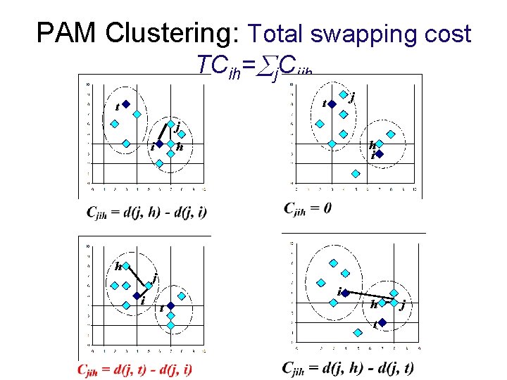
PAM (Partitioning Around Medoids) (1987) • PAM (Kaufman and Rousseeuw, 1987), built in Splus • Use real object to represent the cluster – Select k representative objects arbitrarily – For each pair of non-selected object h and selected object i, calculate the total swapping cost TCih – For each pair of i and h, • If TCih < 0, i is replaced by h • Then assign each non-selected object to the most similar representative object – repeat steps 2 -3 until there is no change

PAM Clustering: Total swapping cost TCih= j. Cjih j t t j i h i h i t h t j

Advantages of PAM? • Pam is more robust than k-means in the presence of noise and outliers because a medoid is less influenced by outliers or other extreme values than a mean. • It produces representative prototypes. • Pam works efficiently for small data sets but does not scale well for large data sets. – O(k(n-k)2 ) for each iteration where n is # of data, k is # of clusters è Sampling based method, CLARA(Clustering LARge Applications)

CLARA (Clustering Large Applications) (1990) • CLARA (Kaufmann and Rousseeuw in 1990) – Built in statistical analysis packages, such as S+ • It draws multiple samples of the data set, applies PAM on each sample, and gives the best clustering as the output • Strength: deals with larger data sets than PAM • Weakness: – Efficiency depends on the sample size – A good clustering based on samples will not necessarily represent a good clustering of the whole data set if the sample is biased

Cluster Analysis • What is Cluster Analysis? • Types of Data in Cluster Analysis • A Categorization of Major Clustering Methods • Partitioning Methods • Hierarchical Methods • Density-Based Methods • Grid-Based Methods • Model-Based Clustering Methods • Outlier Analysis • Summary

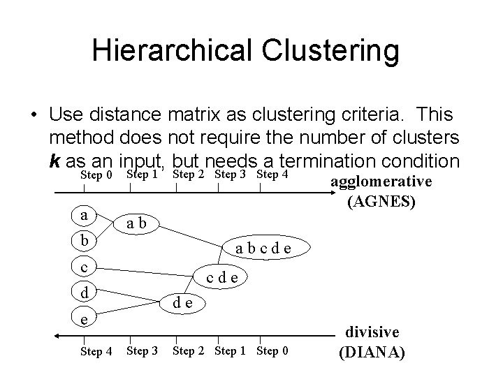
Hierarchical Clustering • Use distance matrix as clustering criteria. This method does not require the number of clusters k as an input, but needs a termination condition Step 0 a b Step 1 Step 2 Step 3 Step 4 ab abcde c cde d de e Step 4 agglomerative (AGNES) Step 3 Step 2 Step 1 Step 0 divisive (DIANA)

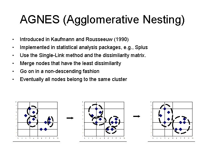
AGNES (Agglomerative Nesting) • Introduced in Kaufmann and Rousseeuw (1990) • Implemented in statistical analysis packages, e. g. , Splus • Use the Single-Link method and the dissimilarity matrix. • Merge nodes that have the least dissimilarity • Go on in a non-descending fashion • Eventually all nodes belong to the same cluster

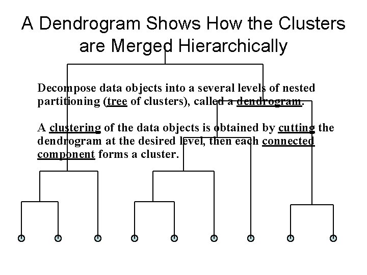
A Dendrogram Shows How the Clusters are Merged Hierarchically Decompose data objects into a several levels of nested partitioning (tree of clusters), called a dendrogram. A clustering of the data objects is obtained by cutting the dendrogram at the desired level, then each connected component forms a cluster.

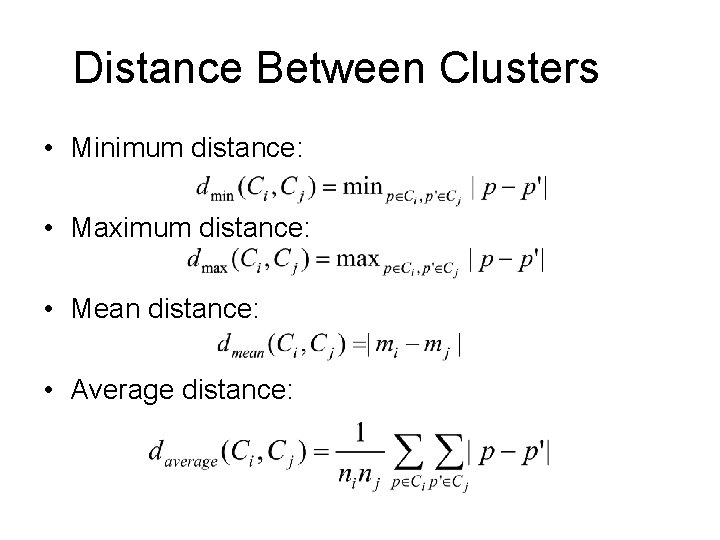
Distance Between Clusters • Minimum distance: • Maximum distance: • Mean distance: • Average distance:

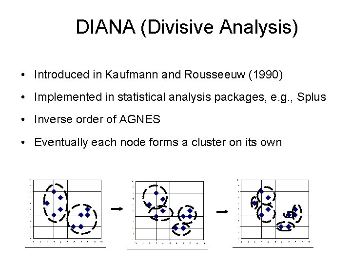
DIANA (Divisive Analysis) • Introduced in Kaufmann and Rousseeuw (1990) • Implemented in statistical analysis packages, e. g. , Splus • Inverse order of AGNES • Eventually each node forms a cluster on its own

More on Hierarchical Clustering Methods • Major weakness of agglomerative clustering methods – do not scale well: time complexity of at least O(n 2), where n is the number of total objects – can never undo what was done previously • Integration of hierarchical with distance-based clustering – BIRCH (1996): uses CF-tree and incrementally adjusts the quality of sub-clusters – CURE (1998): selects well-scattered points from the cluster and then shrinks them towards the center of the cluster by a specified fraction – ROCK – CHAMELEON (1999): hierarchical clustering using dynamic modeling

BIRCH (1996) • Birch: Balanced Iterative Reducing and Clustering using Hierarchies, by Zhang, Ramakrishnan, Livny (SIGMOD’ 96) • Incrementally construct a CF (Clustering Feature) tree, a hierarchical data structure for multiphase clustering – Phase 1: scan DB to build an initial in-memory CF tree (a multi-level compression of the data that tries to preserve the inherent clustering structure of the data) – Phase 2: use an arbitrary clustering algorithm to cluster the leaf nodes of the CF-tree • Scales linearly: finds a good clustering with a single scan and improves the quality with a few additional scans • Weakness: handles only numeric data, and sensitive to the order of the data record.

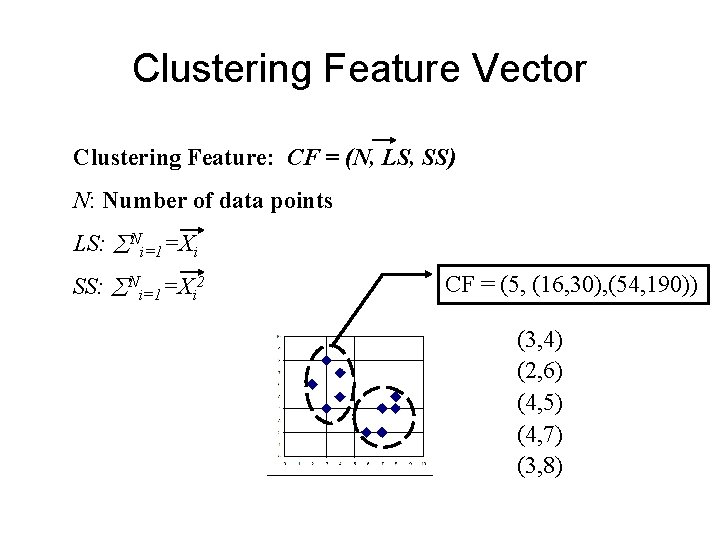
Clustering Feature Vector Clustering Feature: CF = (N, LS, SS) N: Number of data points LS: Ni=1=Xi SS: Ni=1=Xi 2 CF = (5, (16, 30), (54, 190)) (3, 4) (2, 6) (4, 5) (4, 7) (3, 8)

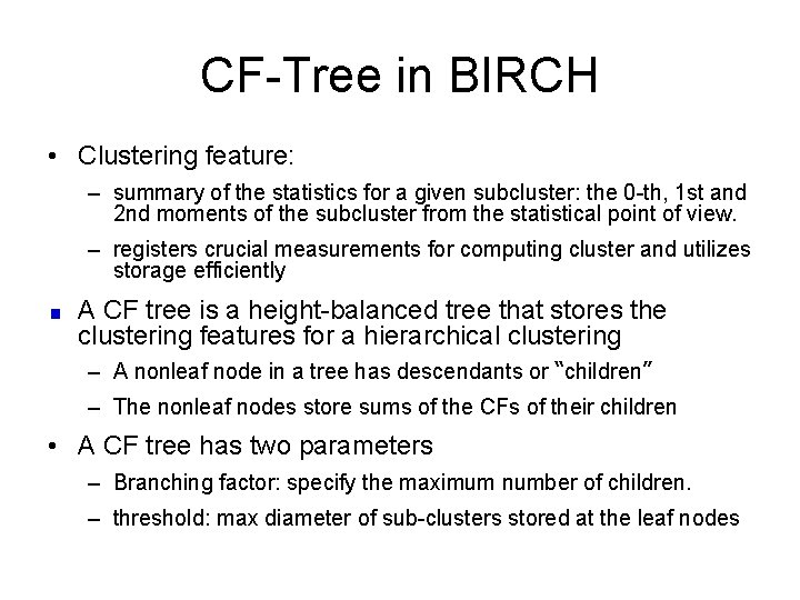
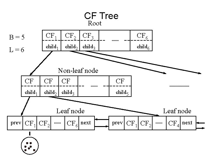
CF-Tree in BIRCH • Clustering feature: – summary of the statistics for a given subcluster: the 0 -th, 1 st and 2 nd moments of the subcluster from the statistical point of view. – registers crucial measurements for computing cluster and utilizes storage efficiently A CF tree is a height-balanced tree that stores the clustering features for a hierarchical clustering – A nonleaf node in a tree has descendants or “children” – The nonleaf nodes store sums of the CFs of their children • A CF tree has two parameters – Branching factor: specify the maximum number of children. – threshold: max diameter of sub-clusters stored at the leaf nodes

CF Tree Root B=5 CF 1 CF 2 CF 3 CF 6 L=6 child 1 child 2 child 3 child 6 CF Non-leaf node CF CF CF child 1 child 2 child 3 child 5 Leaf node prev CF 1 CF 2 CF 6 next Leaf node prev CF 1 CF 2 CF 4 next

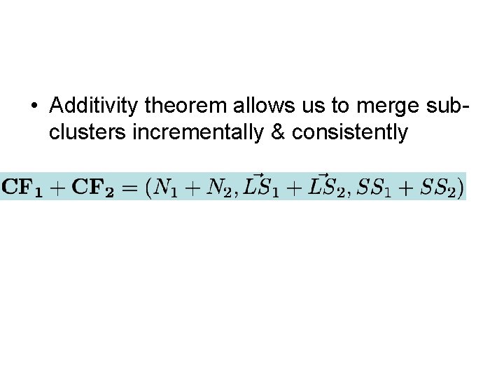
• Additivity theorem allows us to merge subclusters incrementally & consistently

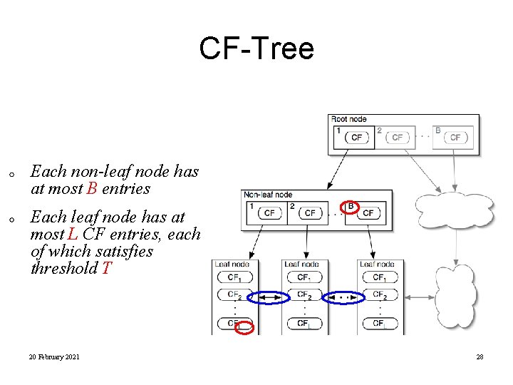
CF-Tree Each non-leaf node has at most B entries Each leaf node has at most L CF entries, each of which satisfies threshold T 20 February 2021 28

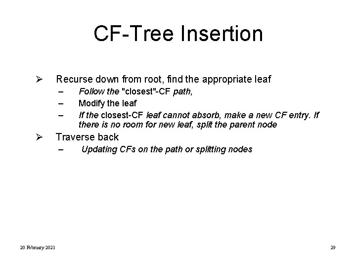
CF-Tree Insertion Ø Recurse down from root, find the appropriate leaf – – – Ø Traverse back – 20 February 2021 Follow the "closest"-CF path, Modify the leaf If the closest-CF leaf cannot absorb, make a new CF entry. If there is no room for new leaf, split the parent node Updating CFs on the path or splitting nodes 29

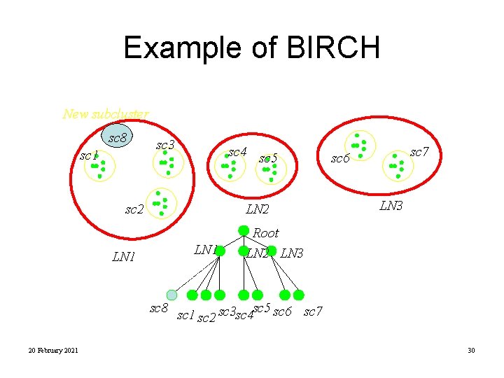
Example of BIRCH New subcluster sc 8 sc 1 sc 3 sc 4 sc 5 sc 2 LN 1 LN 2 LN 1 sc 7 sc 6 LN 3 Root LN 2 LN 3 sc 8 sc 1 sc 5 sc 6 sc 7 sc 3 sc 4 sc 2 20 February 2021 30

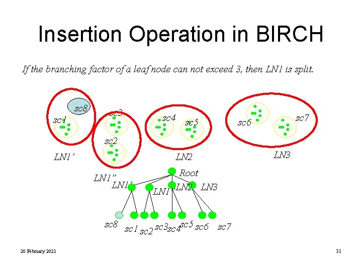
Insertion Operation in BIRCH If the branching factor of a leaf node can not exceed 3, then LN 1 is split. sc 8 sc 1 sc 3 sc 4 sc 5 sc 7 sc 6 sc 2 LN 1’ LN 2 LN 1” LN 1’ LN 3 Root LN 1”LN 2 LN 3 sc 8 sc 1 sc 5 sc 2 sc 3 sc 4 sc 6 sc 7 20 February 2021 31

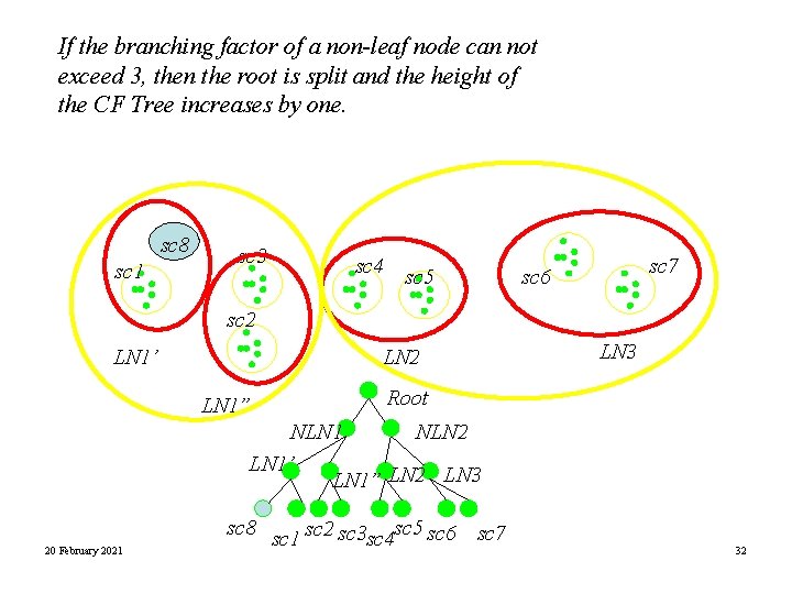
If the branching factor of a non-leaf node can not exceed 3, then the root is split and the height of the CF Tree increases by one. sc 8 sc 1 sc 3 sc 4 sc 5 sc 7 sc 6 sc 2 LN 1’ LN 2 LN 1” LN 3 Root NLN 1 NLN 2 LN 1’ LN 1” LN 2 LN 3 20 February 2021 sc 8 sc 1 sc 2 sc 3 sc 4 sc 5 sc 6 sc 7 32

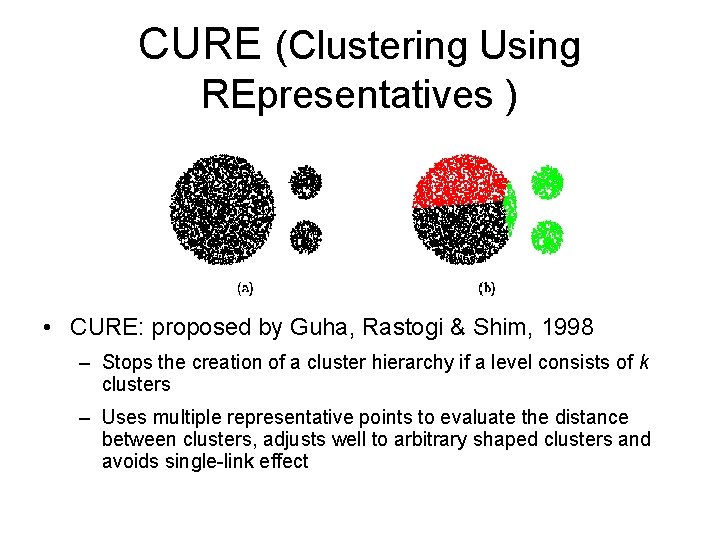
CURE (Clustering Using REpresentatives ) • CURE: proposed by Guha, Rastogi & Shim, 1998 – Stops the creation of a cluster hierarchy if a level consists of k clusters – Uses multiple representative points to evaluate the distance between clusters, adjusts well to arbitrary shaped clusters and avoids single-link effect

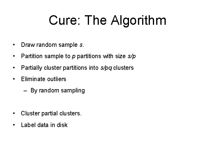
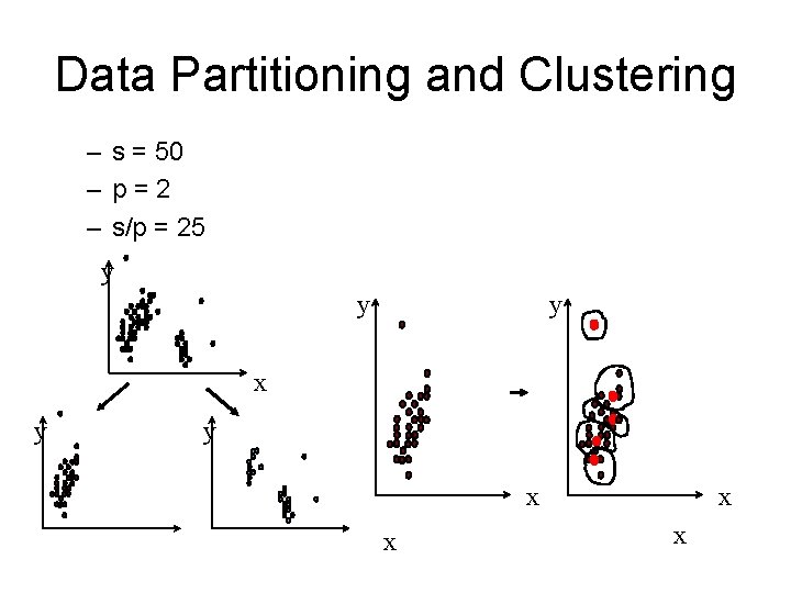
Cure: The Algorithm • Draw random sample s. • Partition sample to p partitions with size s/p • Partially cluster partitions into s/pq clusters • Eliminate outliers – By random sampling • Cluster partial clusters. • Label data in disk

Data Partitioning and Clustering – s = 50 – p=2 – s/p = 25 y y y x x x x

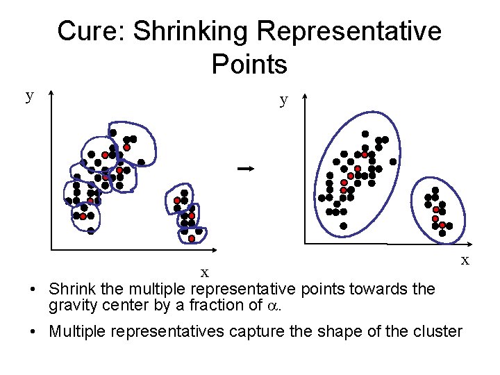
Cure: Shrinking Representative Points y y x • Shrink the multiple representative points towards the gravity center by a fraction of . x • Multiple representatives capture the shape of the cluster

Clustering Categorical Data: ROCK • ROCK: Robust Clustering using lin. Ks, by S. Guha, R. Rastogi, K. Shim (ICDE’ 99). – Use links to measure similarity/proximity – Not distance based • Basic ideas: Similarity function and neighbors:

• Clustering categorical data • No distance measure is used • Algorithm – Draw random sample – Cluster with links – Label data in disk

• An Example Problem Supermarket transactions. • Each datapoint represents the set of items bought by a single customer. • We wish to group customers so that those buying similiar types of items appear in the same group, e. g: • Group A— baby-related: diapers, baby-food, toys. • Group B— expensive imported foodstuffs. • Represent each transaction as a binary vector in which each attribute represents the presence or absence of a particular item in the transaction (boolean).

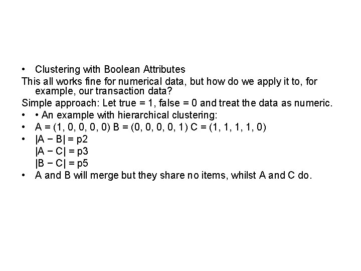
• Clustering with Boolean Attributes This all works fine for numerical data, but how do we apply it to, for example, our transaction data? Simple approach: Let true = 1, false = 0 and treat the data as numeric. • • An example with hierarchical clustering: • A = (1, 0, 0) B = (0, 0, 1) C = (1, 1, 0) • |A − B| = p 2 |A − C| = p 3 |B − C| = p 5 • A and B will merge but they share no items, whilst A and C do.

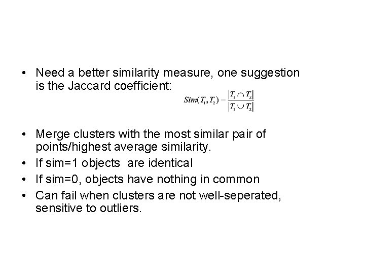
• Need a better similarity measure, one suggestion is the Jaccard coefficient: • Merge clusters with the most similar pair of points/highest average similarity. • If sim=1 objects are identical • If sim=0, objects have nothing in common • Can fail when clusters are not well-seperated, sensitive to outliers.

Neighbours and Links • Need a more global approach that considers the links between points. • Use common neighbours to define links- defined as the number of common neighbours between A and B. • If point A neighbours point C, and point B neighbours point C then the points A and B are linked, even if they are not themselves neighbours. • If two points belong to the same cluster they should have many common neighbours. • If they belong to different clusters they will have few common neighbours.

• We need a way of deciding which points are ‘neighbours’. • Define a similarity function, sim(p 1, p 2), that encodes the level of similarity (’closeness’) between two points. • Then define link(p 1, p 2) to be the number of common neighbours between p 1 and p 2. • The similarity function can be anything— Euclidian distance, the Jaccard coefficient, a similarity table provided by an expert, etc. . . • For supermarket transactions use the Jaccard coefficient. .

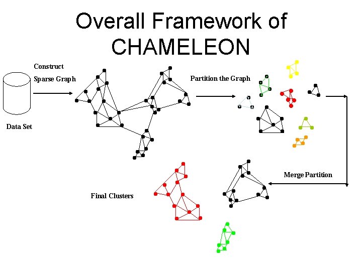
CHAMELEON (Hierarchical clustering using dynamic modeling) • CHAMELEON: by G. Karypis, E. H. Han, and V. Kumar’ 99 • Measures the similarity based on a dynamic model • – Two clusters are merged only if the interconnectivity and closeness (proximity) between two clusters are high relative to the internal interconnectivity of the clusters and closeness of items within the clusters – Cure ignores information about interconnectivity of the objects, Rock ignores information about the closeness of two clusters A two-phase algorithm 1. Use a graph partitioning algorithm: cluster objects into a large number of relatively small sub-clusters 2. Use an agglomerative hierarchical clustering algorithm: find the genuine clusters by repeatedly combining these sub-clusters

Overall Framework of CHAMELEON Construct Partition the Graph Sparse Graph Data Set Merge Partition Final Clusters

Method • Represent objects using KNN graph • Each vertex represents an object and there exist an edge between two objects. • Relative interconnectivity between two clusters is determined • Relative closeness between pair of clusters is determined

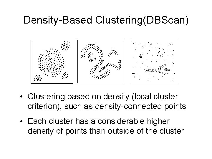
Density-Based Clustering(DBScan) • Clustering based on density (local cluster criterion), such as density-connected points • Each cluster has a considerable higher density of points than outside of the cluster

Density-Based Clustering • Major features: – Discover clusters of arbitrary shape – Handle noise – One scan • Several interesting studies: – – – DBSCAN: Ester, et al. (KDD’ 96) GDBSCAN: Sander, et al. (KDD’ 98) OPTICS: Ankerst, et al (SIGMOD’ 99). DENCLUE: Hinneburg & D. Keim (KDD’ 98) CLIQUE: Agrawal, et al. (SIGMOD’ 98)

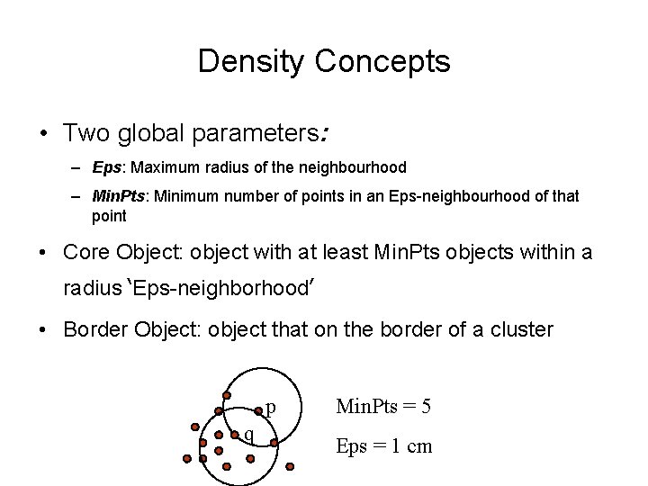
Density Concepts • Two global parameters: – Eps: Maximum radius of the neighbourhood – Min. Pts: Minimum number of points in an Eps-neighbourhood of that point • Core Object: object with at least Min. Pts objects within a radius ‘Eps-neighborhood’ • Border Object: object that on the border of a cluster p q Min. Pts = 5 Eps = 1 cm

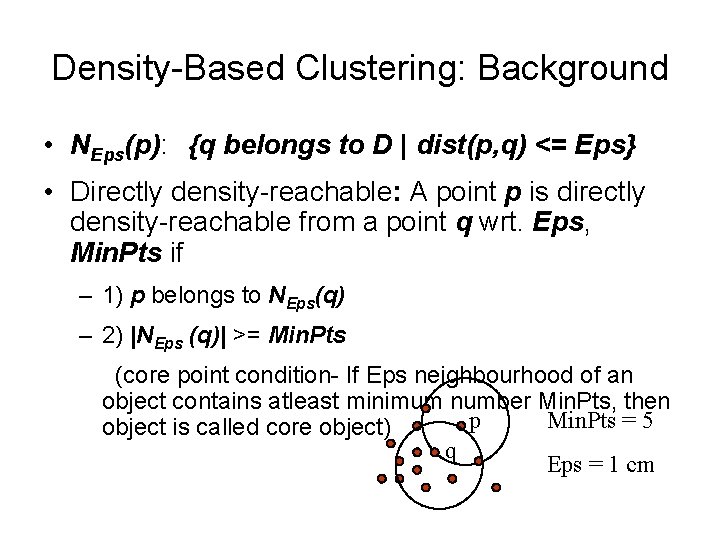
Density-Based Clustering: Background • NEps(p): {q belongs to D | dist(p, q) <= Eps} • Directly density-reachable: A point p is directly density-reachable from a point q wrt. Eps, Min. Pts if – 1) p belongs to NEps(q) – 2) |NEps (q)| >= Min. Pts (core point condition- If Eps neighbourhood of an object contains atleast minimum number Min. Pts, then p Min. Pts = 5 object is called core object) q Eps = 1 cm

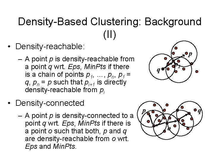
Density-Based Clustering: Background (II) • Density-reachable: p – A point p is density-reachable from a point q wrt. Eps, Min. Pts if there is a chain of points p 1, …, pn, p 1 = q, pn = p such that pi+1 is directly density-reachable from pi • Density-connected – A point p is density-connected to a point q wrt. Eps, Min. Pts if there is a point o such that both, p and q are density-reachable from o wrt. Eps and Min. Pts. p 1 q p q o

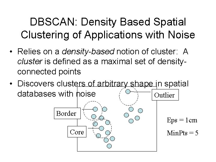
DBSCAN: Density Based Spatial Clustering of Applications with Noise • Relies on a density-based notion of cluster: A cluster is defined as a maximal set of densityconnected points • Discovers clusters of arbitrary shape in spatial databases with noise Outlier Border Core Eps = 1 cm Min. Pts = 5

DBSCAN: The Algorithm (1) – Arbitrary select a point p – Retrieve all points density-reachable from p wrt Eps and Min. Pts. – If p is a core point, a cluster is formed. – If p is a border point, no points are densityreachable from p and DBSCAN visits the next point of the database. – Continue the process until all of the points have been processed.

Techniques for Grid-Based Clustering The following are some techniques that are used to perform Grid-Based Clustering: – CLIQUE (CLustering In QUest. ) – STING (STatistical Information Grid. ) – Wave. Cluster

Looking at CLIQUE as an Example • CLIQUE is used for the clustering of highdimensional data present in large tables. By high-dimensional data we mean records that have many attributes. • CLIQUE identifies the dense units in the subspaces of high dimensional data space, and uses these subspaces to provide more efficient clustering.

Definitions That Need to Be Known • Unit : After forming a grid structure on the space, each rectangular cell is called a Unit. • Dense: A unit is dense, if the fraction of total data points contained in the unit exceeds the input model parameter. • Cluster: A cluster is defined as a maximal set of connected dense units.

How Does CLIQUE Work? • Let us say that we have a set of records that we would like to cluster in terms of nattributes. • So, we are dealing with an n-dimensional space. • MAJOR STEPS : – CLIQUE partitions each subspace that has dimension 1 into the same number of equal length intervals. – Using this as basis, it partitions the ndimensional data space into non-overlapping rectangular units.

CLIQUE: Major Steps (Cont. ) – Now CLIQUE’S goal is to identify the dense ndimensional units. – It does this in the following way: – CLIQUE finds dense units of higher dimensionality by finding the dense units in the subspaces. – So, for example if we are dealing with a 3 -dimensional space, CLIQUE finds the dense units in the 3 related PLANES (2 -dimensional subspaces. ) – It then intersects the extension of the subspaces representing the dense units to form a candidate search space in which dense units of higher dimensionality would exist.

CLIQUE: Major Steps. (Cont. ) – Each maximal set of connected dense units is considered a cluster. – Using this definition, the dense units in the subspaces are examined in order to find clusters in the subspaces. – The information of the subspaces is then used to find clusters in the n-dimensional space. – It must be noted that all cluster boundaries are either horizontal or vertical. This is due to the nature of the rectangular grid cells.

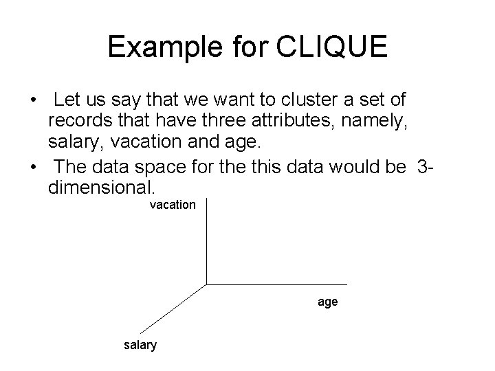
Example for CLIQUE • Let us say that we want to cluster a set of records that have three attributes, namely, salary, vacation and age. • The data space for the this data would be 3 dimensional. vacation age salary

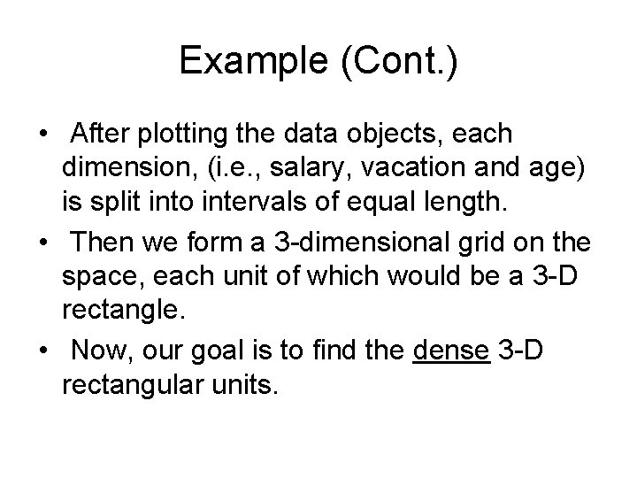
Example (Cont. ) • After plotting the data objects, each dimension, (i. e. , salary, vacation and age) is split into intervals of equal length. • Then we form a 3 -dimensional grid on the space, each unit of which would be a 3 -D rectangle. • Now, our goal is to find the dense 3 -D rectangular units.

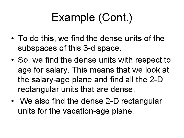
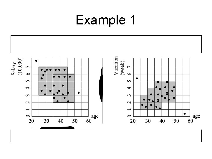
Example (Cont. ) • To do this, we find the dense units of the subspaces of this 3 -d space. • So, we find the dense units with respect to age for salary. This means that we look at the salary-age plane and find all the 2 -D rectangular units that are dense. • We also find the dense 2 -D rectangular units for the vacation-age plane.

Example 1

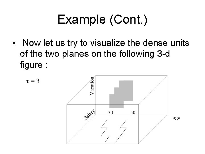
Example (Cont. ) • Now let us try to visualize the dense units of the two planes on the following 3 -d figure :

Example (Cont. ) • We can extend the dense areas in the vacationage plane inwards. • We can extend the dense areas in the salaryage plane upwards. • The intersection of these two spaces would give us a candidate search space in which 3 dimensional dense units exist. • We then find the dense units in the salaryvacation plane and we form an extension of the subspace that represents these dense units.

Example (Cont. ) • Now, we perform an intersection of the candidate search space with the extension of the dense units of the salary-vacation plane, in order to get all the 3 -d dense units. • So, What was the main idea? • We used the dense units in subspaces in order to find the dense units in the 3 dimensional space. • After finding the dense units, it is very easy to find clusters.

Reflecting upon CLIQUE • Why does CLIQUE confine its search for dense units in high dimensions to the intersection of dense units in subspaces? • Because the Apriori property employs prior knowledge of the items in the search space so that portions of the space can be pruned. • The property for CLIQUE (Apriori property)says that if a k-dimensional unit is dense then so are its projections in the (k-1) dimensional space.

Strength and Weakness of CLIQUE • Strength – It automatically finds subspaces of the highest dimensionality such that high density clusters exist in those subspaces. – It is quite efficient. – It is insensitive to the order of records in input and does not presume some canonical data distribution. – It scales linearly with the size of input and has good scalability as the number of dimensions in the data increases. • Weakness – The accuracy of the clustering result may be degraded at the expense of simplicity of this method.

Model-Based Clustering • What is model-based clustering? – Attempt to optimize the fit between the given data and some mathematical model – Based on the assumption: Data are generated by a mixture of underlying probability distribution • Typical methods – Statistical approach • EM (Expectation maximization), Auto. Class – Machine learning approach • COBWEB, CLASSIT – Neural network approach • SOM (Self-Organizing Feature Map)

EM — Expectation Maximization • EM — A popular iterative refinement algorithm • An extension to k-means – Assign each object to a cluster according to a weight (prob. distribution) – New means are computed based on weighted measures (no strict boundaries between clusters) • General idea – Starts with an initial estimate of the parameter vector (parameters of mixture model) – Iteratively rescores the patterns against the mixture density produced by the parameter vector – The rescored patterns are used to update the parameter estimates – Patterns belong to the same cluster, if they are placed by their scores in a particular component

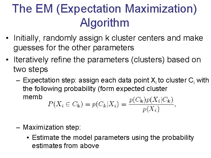
The EM (Expectation Maximization) Algorithm • Initially, randomly assign k cluster centers and make guesses for the other parameters • Iteratively refine the parameters (clusters) based on two steps – Expectation step: assign each data point Xi to cluster Ci with the following probability (form expected cluster memberships of Xi ) – Maximization step: • Estimate the model parameters using the probability estimates from above

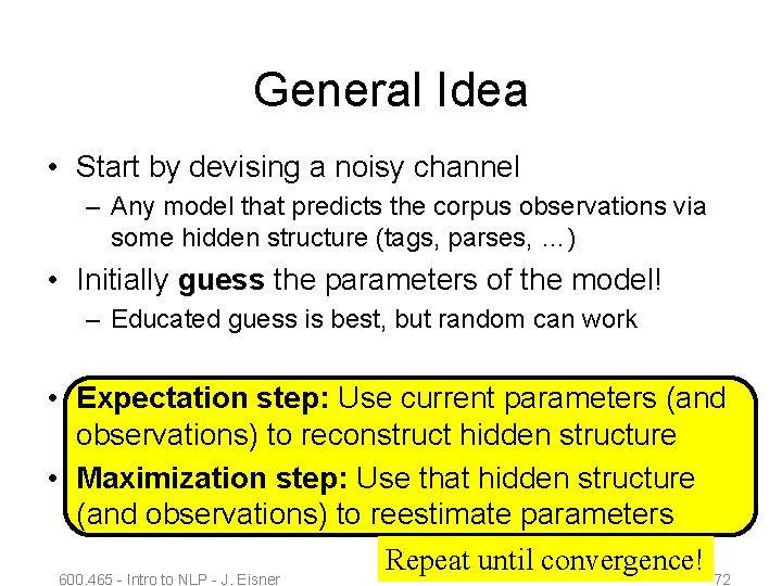
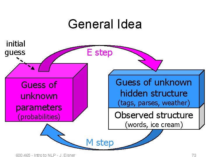
General Idea • Start by devising a noisy channel – Any model that predicts the corpus observations via some hidden structure (tags, parses, …) • Initially guess the parameters of the model! – Educated guess is best, but random can work • Expectation step: Use current parameters (and observations) to reconstruct hidden structure • Maximization step: Use that hidden structure (and observations) to reestimate parameters Repeat until convergence! 600. 465 - Intro to NLP - J. Eisner 72

General Idea initial guess E step Guess of unknown hidden structure Guess of unknown parameters (tags, parses, weather) Observed structure (probabilities) (words, ice cream) M step 600. 465 - Intro to NLP - J. Eisner 73

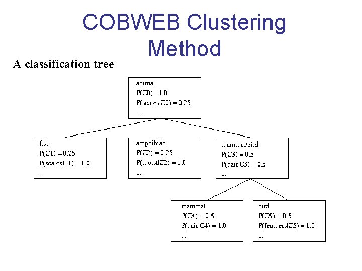
Conceptual Clustering • Conceptual clustering (clustering + characterization) – A form of clustering in machine learning – Produces a classification scheme for a set of unlabeled objects – Finds characteristic description for each concept (class) • COBWEB (Fisher’ 87) – A popular, simple method of incremental conceptual learning – Creates a hierarchical clustering in the form of a classification tree – Each node refers to a concept and contains a probabilistic description of that concept –> main difference from decision trees

COBWEB Clustering Method A classification tree

More on Conceptual Clustering • Limitations of COBWEB – The assumption that the attributes are independent of each other is often too strong - correlation may exist – Not suitable for clustering large database data – skewed tree and expensive probability distributions (time and space complexity depends not only on the number of attributes but also on the number of values for these attributes) • CLASSIT – an extension of COBWEB for incremental clustering of continuous data – suffers similar problems as COBWEB • Auto. Class (Cheeseman and Stutz, 1996) – Uses Bayesian statistical analysis to estimate the number of clusters – Popular in industry

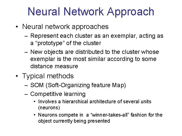
Neural Network Approach • Neural network approaches – Represent each cluster as an exemplar, acting as a “prototype” of the cluster – New objects are distributed to the cluster whose exemplar is the most similar according to some distance measure • Typical methods – SOM (Soft-Organizing feature Map) – Competitive learning • Involves a hierarchical architecture of several units (neurons) • Neurons compete in a “winner-takes-all” fashion for the object currently being presented

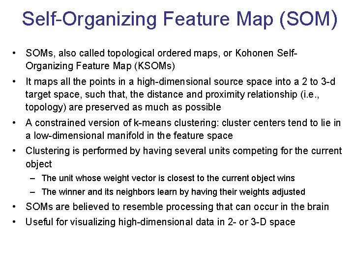
Self-Organizing Feature Map (SOM) • SOMs, also called topological ordered maps, or Kohonen Self. Organizing Feature Map (KSOMs) • It maps all the points in a high-dimensional source space into a 2 to 3 -d target space, such that, the distance and proximity relationship (i. e. , topology) are preserved as much as possible • A constrained version of k-means clustering: cluster centers tend to lie in a low-dimensional manifold in the feature space • Clustering is performed by having several units competing for the current object – The unit whose weight vector is closest to the current object wins – The winner and its neighbors learn by having their weights adjusted • SOMs are believed to resemble processing that can occur in the brain • Useful for visualizing high-dimensional data in 2 - or 3 -D space

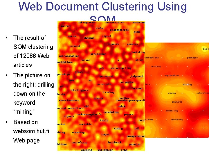
Web Document Clustering Using SOM • The result of SOM clustering of 12088 Web articles • The picture on the right: drilling down on the keyword “mining” • Based on websom. hut. fi Web page

Agenda • What is Cluster Analysis? • Types of Data in Cluster Analysis • A Categorization of Major Clustering Methods • Partitioning Methods • Hierarchical Methods • Density-Based Methods • Grid-Based Methods • Model-Based Clustering Methods • Outlier Analysis • Summary

What Is Outlier Discovery? • What are outliers? – The set of objects are considerably dissimilar from the remainder of the data – Example: Sports: Michael Jordan, Wayne Gretzky, . . . • Problem – Find top n outlier points • Applications: – – Credit card fraud detection Telecom fraud detection Customer segmentation Medical analysis

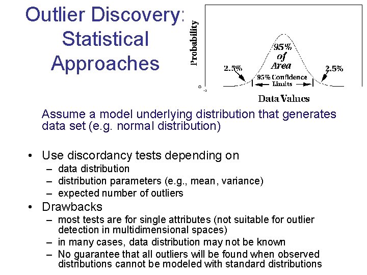
Outlier Discovery: Statistical Approaches Assume a model underlying distribution that generates data set (e. g. normal distribution) • Use discordancy tests depending on – data distribution – distribution parameters (e. g. , mean, variance) – expected number of outliers • Drawbacks – most tests are for single attributes (not suitable for outlier detection in multidimensional spaces) – in many cases, data distribution may not be known – No guarantee that all outliers will be found when observed distributions cannot be modeled with standard distributions

• Cases of alternative distribution • Inherent alternative distribution • Mixture alternative distribution • Slippage alternative distribution • Procedures for detecting outliers • Block procedure • Consecutive or sequential procedures – inside outside test

Outlier Discovery: Distance-Based Approach • Introduced to overcome the main limitations of statistical methods – We need multi-dimensional analysis without knowing data distribution. • Distance-based outlier: an object that does not have “enough” neighbors: • Algorithms for mining distance-based outliers – Index-based algorithm (uses multidimensional indexing structures( R-trees etc) to search for neighbors) – Nested-loop algorithm (tries to minimize # of I/Os) – Cell-based algorithm (partitions the space into cells)

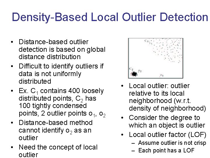
Density-Based Local Outlier Detection • Distance-based outlier detection is based on global distance distribution • Difficult to identify outliers if data is not uniformly distributed • Ex. C 1 contains 400 loosely distributed points, C 2 has 100 tightly condensed points, 2 outlier points o 1, o 2 • Distance-based method cannot identify o 2 as an outlier • Need the concept of local outlier • Local outlier: outlier relative to its local neighborhood (w. r. t. density of neighborhood) • Consider the degree to which an object is outlier • Local outlier factor (LOF) – Assume outlier is not crisp – Each point has a LOF

Outlier Discovery: Deviation. Based Approach • Identifies outliers by examining the main characteristics of objects in a group • Objects that “deviate” from this description are considered outliers • sequential exception technique – simulates the way in which humans can distinguish unusual objects from among a series of supposedly like objects • OLAP data cube technique – uses data cubes to identify regions of anomalies in large multidimensional data

GA Quick Overview • Developed: USA in the 1970’s • Early names: J. Holland, K. De. Jong, D. Goldberg • Typically applied to: – discrete optimization • Attributed features: – not too fast – good heuristic for combinatorial problems • Special Features: – Traditionally emphasizes combining information from good parents (crossover) – many variants, e. g. , reproduction models, operators

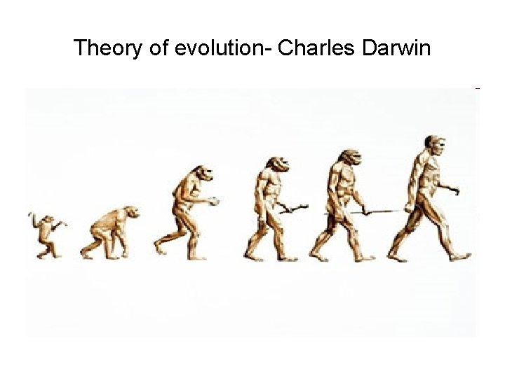
Theory of evolution- Charles Darwin

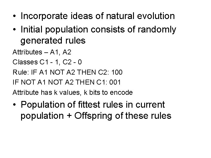
• Incorporate ideas of natural evolution • Initial population consists of randomly generated rules Attributes – A 1, A 2 Classes C 1 - 1, C 2 - 0 Rule: IF A 1 NOT A 2 THEN C 2: 100 IF NOT A 1 NOT A 2 THEN C 1: 001 Attribute has k values, k bits to encode • Population of fittest rules in current population + Offspring of these rules

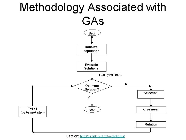
Methodology Associated with GAs Begi n Initialize population Evaluate Solutions T =0 (first step) Optimum Solution? N Selection Y T=T+1 (go to next step) Stop Crossover Mutation Citation: http: //cs. felk. cvut. cz/~xobitko/ga/

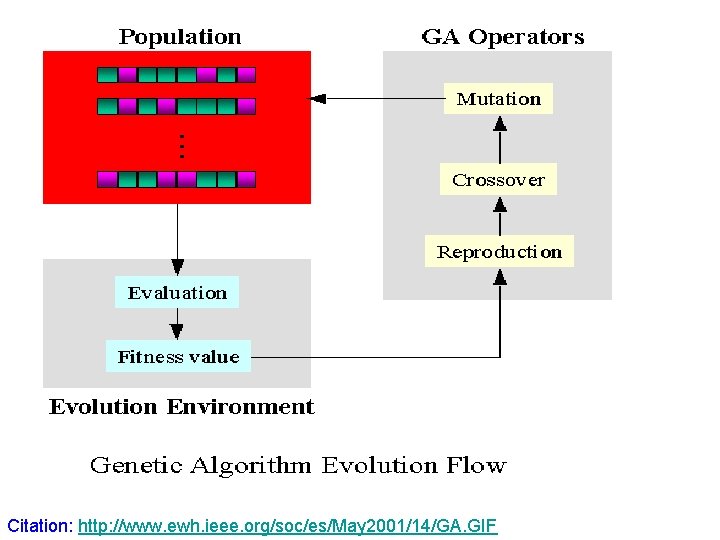
Citation: http: //www. ewh. ieee. org/soc/es/May 2001/14/GA. GIF

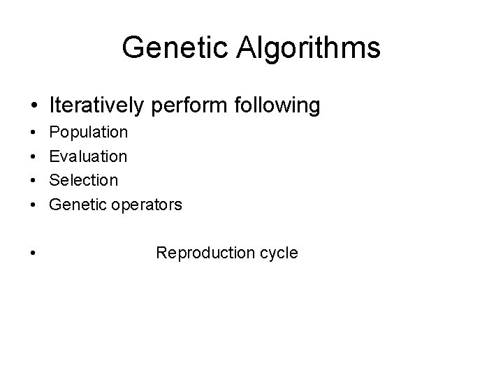
Genetic Algorithms • Iteratively perform following • • • Population Evaluation Selection Genetic operators Reproduction cycle

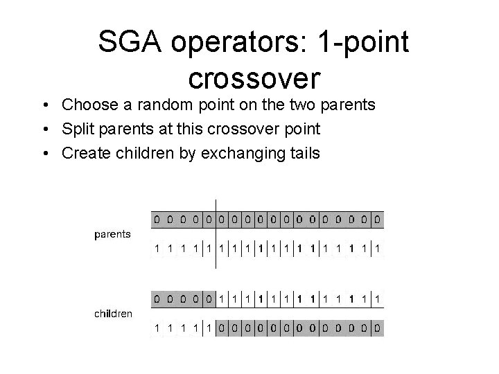
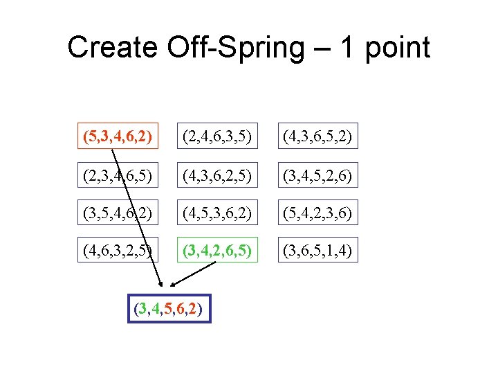
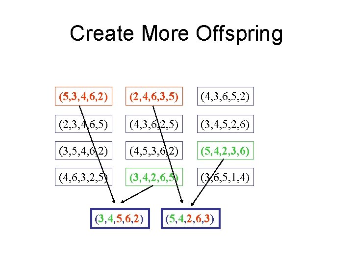
SGA operators: 1 -point crossover • Choose a random point on the two parents • Split parents at this crossover point • Create children by exchanging tails

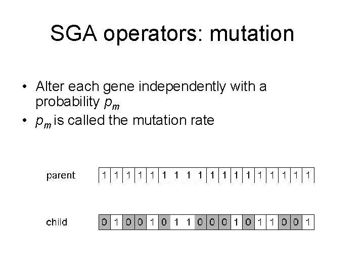
SGA operators: mutation • Alter each gene independently with a probability pm • pm is called the mutation rate

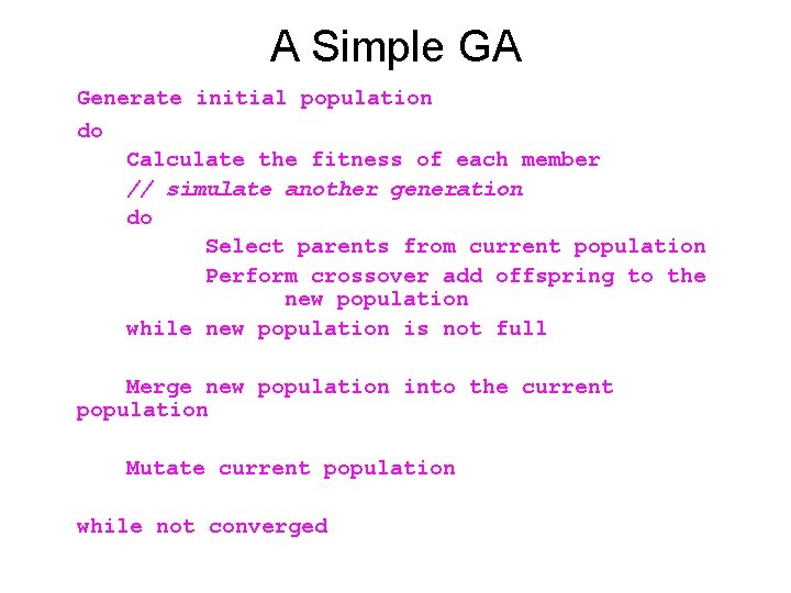
A Simple GA Generate initial population do Calculate the fitness of each member // simulate another generation do Select parents from current population Perform crossover add offspring to the new population while new population is not full Merge new population into the current population Mutate current population while not converged

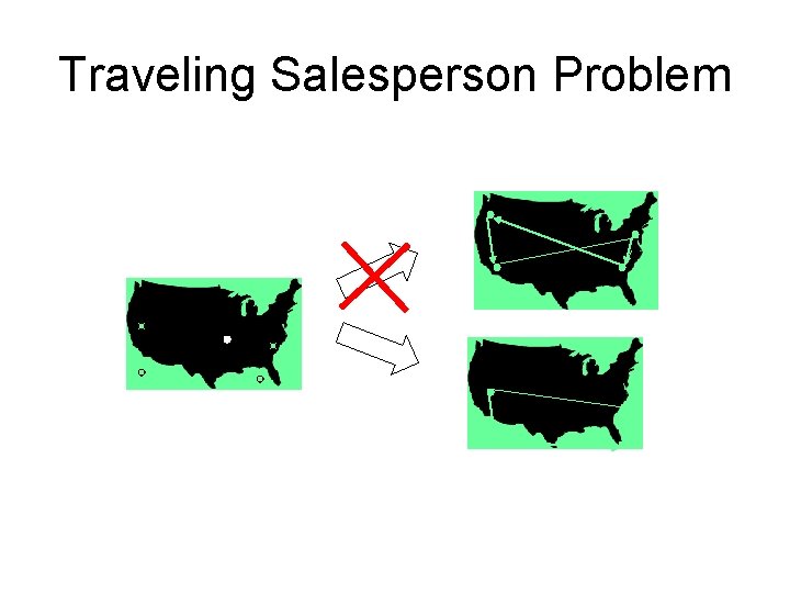
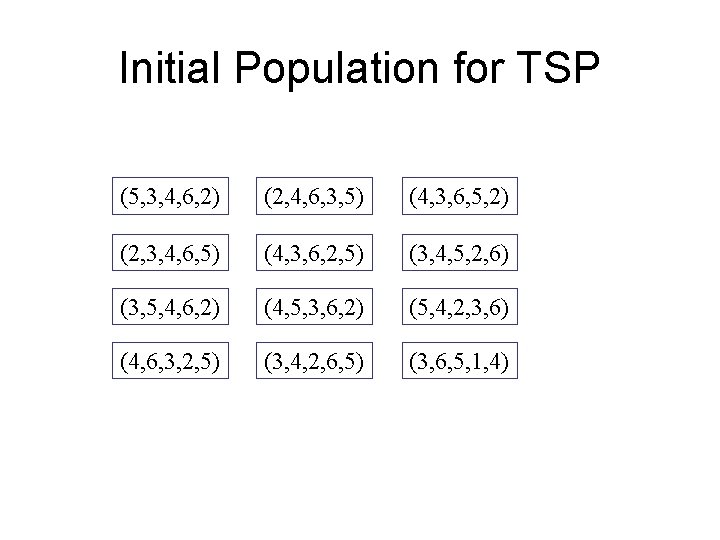
Traveling Salesperson Problem

Initial Population for TSP (5, 3, 4, 6, 2) (2, 4, 6, 3, 5) (4, 3, 6, 5, 2) (2, 3, 4, 6, 5) (4, 3, 6, 2, 5) (3, 4, 5, 2, 6) (3, 5, 4, 6, 2) (4, 5, 3, 6, 2) (5, 4, 2, 3, 6) (4, 6, 3, 2, 5) (3, 4, 2, 6, 5) (3, 6, 5, 1, 4)

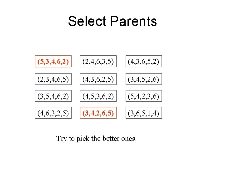
Select Parents (5, 3, 4, 6, 2) (2, 4, 6, 3, 5) (4, 3, 6, 5, 2) (2, 3, 4, 6, 5) (4, 3, 6, 2, 5) (3, 4, 5, 2, 6) (3, 5, 4, 6, 2) (4, 5, 3, 6, 2) (5, 4, 2, 3, 6) (4, 6, 3, 2, 5) (3, 4, 2, 6, 5) (3, 6, 5, 1, 4) Try to pick the better ones.

Create Off-Spring – 1 point (5, 3, 4, 6, 2) (2, 4, 6, 3, 5) (4, 3, 6, 5, 2) (2, 3, 4, 6, 5) (4, 3, 6, 2, 5) (3, 4, 5, 2, 6) (3, 5, 4, 6, 2) (4, 5, 3, 6, 2) (5, 4, 2, 3, 6) (4, 6, 3, 2, 5) (3, 4, 2, 6, 5) (3, 6, 5, 1, 4) (3, 4, 5, 6, 2)

Create More Offspring (5, 3, 4, 6, 2) (2, 4, 6, 3, 5) (4, 3, 6, 5, 2) (2, 3, 4, 6, 5) (4, 3, 6, 2, 5) (3, 4, 5, 2, 6) (3, 5, 4, 6, 2) (4, 5, 3, 6, 2) (5, 4, 2, 3, 6) (4, 6, 3, 2, 5) (3, 4, 2, 6, 5) (3, 6, 5, 1, 4) (3, 4, 5, 6, 2) (5, 4, 2, 6, 3)

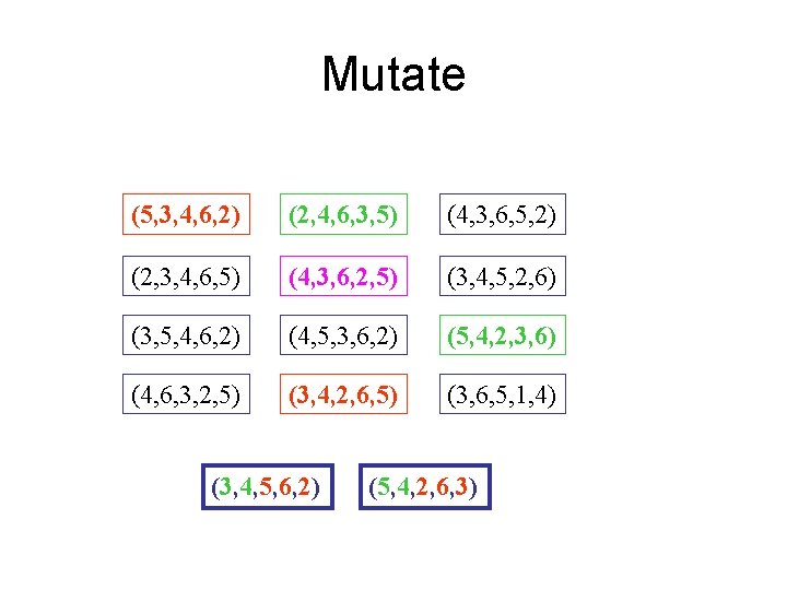
Mutate (5, 3, 4, 6, 2) (2, 4, 6, 3, 5) (4, 3, 6, 5, 2) (2, 3, 4, 6, 5) (4, 3, 6, 2, 5) (3, 4, 5, 2, 6) (3, 5, 4, 6, 2) (4, 5, 3, 6, 2) (5, 4, 2, 3, 6) (4, 6, 3, 2, 5) (3, 4, 2, 6, 5) (3, 6, 5, 1, 4) (3, 4, 5, 6, 2) (5, 4, 2, 6, 3)

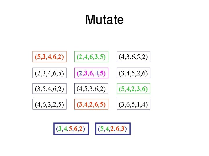
Mutate (5, 3, 4, 6, 2) (2, 4, 6, 3, 5) (4, 3, 6, 5, 2) (2, 3, 4, 6, 5) (2, 3, 6, 4, 5) (3, 4, 5, 2, 6) (3, 5, 4, 6, 2) (4, 5, 3, 6, 2) (5, 4, 2, 3, 6) (4, 6, 3, 2, 5) (3, 4, 2, 6, 5) (3, 6, 5, 1, 4) (3, 4, 5, 6, 2) (5, 4, 2, 6, 3)

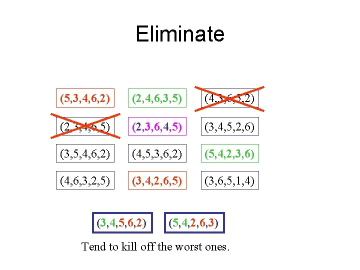
Eliminate (5, 3, 4, 6, 2) (2, 4, 6, 3, 5) (4, 3, 6, 5, 2) (2, 3, 4, 6, 5) (2, 3, 6, 4, 5) (3, 4, 5, 2, 6) (3, 5, 4, 6, 2) (4, 5, 3, 6, 2) (5, 4, 2, 3, 6) (4, 6, 3, 2, 5) (3, 4, 2, 6, 5) (3, 6, 5, 1, 4) (3, 4, 5, 6, 2) (5, 4, 2, 6, 3) Tend to kill off the worst ones.

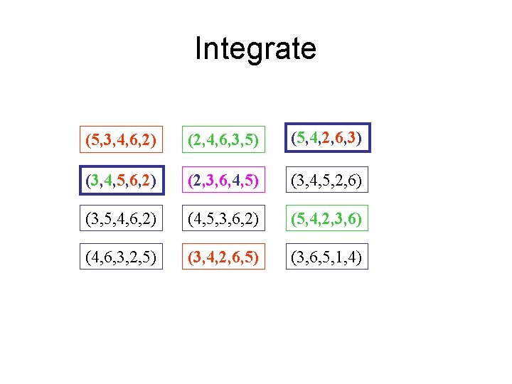
Integrate (5, 3, 4, 6, 2) (2, 4, 6, 3, 5) (5, 4, 2, 6, 3) (3, 4, 5, 6, 2) (2, 3, 6, 4, 5) (3, 4, 5, 2, 6) (3, 5, 4, 6, 2) (4, 5, 3, 6, 2) (5, 4, 2, 3, 6) (4, 6, 3, 2, 5) (3, 4, 2, 6, 5) (3, 6, 5, 1, 4)

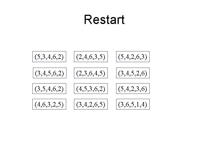
Restart (5, 3, 4, 6, 2) (2, 4, 6, 3, 5) (5, 4, 2, 6, 3) (3, 4, 5, 6, 2) (2, 3, 6, 4, 5) (3, 4, 5, 2, 6) (3, 5, 4, 6, 2) (4, 5, 3, 6, 2) (5, 4, 2, 3, 6) (4, 6, 3, 2, 5) (3, 4, 2, 6, 5) (3, 6, 5, 1, 4)