Cluster Analysis 3 Application Market Segmentation Benefit Segmentation
")
Cluster Analysis (군집 분석)

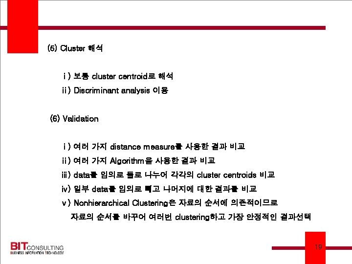
 Application ⅰ) ⅱ) ⅲ) ⅳ) ⅴ) Market Segmentation /Benefit Segmentation 구매행동 이해 :")
(3) Application ⅰ) ⅱ) ⅲ) ⅳ) ⅴ) Market Segmentation /Benefit Segmentation 구매행동 이해 : 동질구매집단 분류를 통한 특성 파악 신제품 기회요인 도출 : brand와 Product를 clustering Test market 선정 Data 축소 (4) Cluster Vs. Factor Analysis cluster : 대상 분류 Factor : 변수(variable) 분류 (5) Cluster Vs. Discriminant Analysis - Object Classification Cluster : Cluster나 Group에 대한 사전 정보(분류기준)가 없는 경우 (독립 관계 분석) Discriminant : Cluster나 Group에 대한 사전 정보가 있는 경우 (종속 관계 분석) 12/3/2020 2

Cluster Analysis 방법 Formulating the problem Selecting a Distance Measure Selecting a Clustering Procedure Deciding on the Number of Clusters Interpreting and Profiling Clusters Assessing the Validity of Clustering 12/3/2020 3

▣ Basic Concept ● An Ideal Clustering Situation ● A Practical Clustering Situation ● ● ● ● Variable 1 ● ● ● ● ● ● ● ● ● ● ● ● ● ● ● ● ● ● ● ● ● ● ● ● ● ● Variable 2 12/3/2020 Variable 2 4

 하여 scale상의 차이로 발생된 bias를")
Normalized distance function : Raw data를 Normalization (Mean=0, Variance=1) 하여 scale상의 차이로 발생된 bias를 해결한 Euclidean distance ② Squared Euclidean distance Dij = ∑(Xik - Xjk)2 i=1 An example of Euclidean distance between two objects measured on two variables – X and Y. Y ● (X 2 -Y 2) (Y 2 -Y 1) Object 1 ● (X 1 -Y 1) X Distance = 12/3/2020 2 (X 2 -X 1) + (Y 2 -Y 1) 2 6
![③ City-block distance (Manhattan distance) r dijc = ∑ Xik - Xjk i=1 [문제점]](http://slidetodoc.com/presentation_image_h/d957ca98c9afee004876f182c0a7d673/image-8.jpg "③ City-block distance (Manhattan distance) r dijc = ∑ Xik - Xjk i=1 [문제점]")
③ City-block distance (Manhattan distance) r dijc = ∑ Xik - Xjk i=1 [문제점] ⅰ) 변수간에 correlation이 없다는 가정 ⅱ) Characteristic을 측정하는 단위(Scales)이 상이성이 가능 -------------------------------Object Purchase Commercial Distance Citi-block Probability(%) Viewing Time(min) (second) -------------------------------A 60 3. 0 AB 25. 25 61 B 65 3. 5 AC 10. 00 153 C 64 4. 0 BC 4. 25 40 ------------------------------- 12/3/2020 7
 Standard Deviation으로 scaling해서 data 표준화 ⅱ) intercorrelation을 조정하기 위해서 within-group")
④ Mahalanobis distance ⅰ) Standard Deviation으로 scaling해서 data 표준화 ⅱ) intercorrelation을 조정하기 위해서 within-group variance-covariance 합산하는 접근 방식 ⅲ) 변수간에 서로 correlated 되었을 때 가장 적합 ⑤ Minkowski distance dij. M = [∑(Xik - Xjk)p]1/r 12/3/2020 8
 Clustering Algorithms Clustering Procedures Nonhierarchical Hierarchical Divisive Hierarchical Sequential Threshold Linkage Methods Variance")
(3) Clustering Algorithms Clustering Procedures Nonhierarchical Hierarchical Divisive Hierarchical Sequential Threshold Linkage Methods Variance Methods Parallel Threshold Optimizing Partitioning Centroid Methods Ward’s Method Single Linkage 12/3/2020 Complete Linkage Average Linkage 9
 계층적 군집방법 (Hierarchical Cluster Procedure) ① Agglomerative Procedure : 한 개의 대상에서 출발하여,")
1) 계층적 군집방법 (Hierarchical Cluster Procedure) ① Agglomerative Procedure : 한 개의 대상에서 출발하여, 주위의 대상이나 cluster를 군집화하여 최종적으로 1개의 cluster로 만드는 방법 ⅰ) Single Linkage : minimum distance rule 군집이나 대상간의 최소거리로 군집화 ⅱ) Complete Linkage : maximum distance rule ⅲ) Average Linkage ⅳ) Ward's Method : W ● Within-cluster variance minimization rule ● Within-cluster distance의 전체 sum of square의 증가가 최소가 되게 cluster ⅴ) Centroid Method ● 대상이나 cluster의 Centroid(mean)간의 거리 최소화 ● 단점 : Metric data에만 적용 가능 12/3/2020 10

② Decisive Method : 큰 한 개의 cluster로 부터 분리시켜 가는 방법 Dendrogram illustrating hierarchical clustering. 01 Observation number 02 03 04 05 06 07 08 1 12/3/2020 2 3 4 5 6 7 11
![[Single Linkage : 단일기준 결합 방식] A 1. 5 1. 2 D A D](http://slidetodoc.com/presentation_image_h/d957ca98c9afee004876f182c0a7d673/image-13.jpg "[Single Linkage : 단일기준 결합 방식] A 1. 5 1. 2 D A D")
[Single Linkage : 단일기준 결합 방식] A 1. 5 1. 2 D A D 1. 55 1. 4 B B 1. 3 C C [Complete Linkage : 완전기준 결합방식] A A 1. 55 D D B C 12/3/2020 B C 12
![[Average Linkage : 평균기준 결합방식] A A 1. 45 D D 1. 425 B](http://slidetodoc.com/presentation_image_h/d957ca98c9afee004876f182c0a7d673/image-14.jpg "[Average Linkage : 평균기준 결합방식] A A 1. 45 D D 1. 425 B")
[Average Linkage : 평균기준 결합방식] A A 1. 45 D D 1. 425 B B C 12/3/2020 C 13
![[Ward Method] ● ● ● [Centroid Method] ● ● ● 12/3/2020 ● ● ●](http://slidetodoc.com/presentation_image_h/d957ca98c9afee004876f182c0a7d673/image-15.jpg "[Ward Method] ● ● ● [Centroid Method] ● ● ● 12/3/2020 ● ● ●")
[Ward Method] ● ● ● [Centroid Method] ● ● ● 12/3/2020 ● ● ● 14
 비계층적 군집방법 (Nonhierarchical Clustering Procedures) = k-means clustering ⅰ) Sequential threshold procedure ①")
2) 비계층적 군집방법 (Nonhierarchical Clustering Procedures) = k-means clustering ⅰ) Sequential threshold procedure ① 하나의 cluster center를 선택하고 미리 산정된 거리 내에 있는 모든 대상을 그 cluster안에 포함시킨다. ② 두 번째 cluster center를 선택하고 미리 산정된 거리 내에 있는 모든 대상을 그 cluster안에 포함시킨다. ⅱ) parallel threshold Procedure ① 초기에 여러 개의 cluster center를 선정하여 가장 가까운 center 로 대상을 포함시킨다 ② threshold 거리는 조절될 수 있다 ⅲ) Optimizing Partitioning Method : 전체적인 optimizing criterion (e. g. , within-cluster distance의 평균)에 따라 나중에 대상을 cluster별로 재편입 시킬 수 있다 12/3/2020 15

▣ Nonhierarchical Clustering의 단점 ① 사전에 cluster 수를 결정해야 한다 ② Cluster Center 선정이 임의적이다 ③ 결과가 data의 순서에 의존적이다 ▣ Nonhierarchical Clustering의 장점 ① center 선정에 있어서 nonrandorn ② Clustering 속도가 빠르다 12/3/2020 16
 군집방법 선택 : Hierarchical Vs. Nonhierarchical ⅰ) Hierarchical + Ward's Method + average")
3) 군집방법 선택 : Hierarchical Vs. Nonhierarchical ⅰ) Hierarchical + Ward's Method + average linkage ⇒ 처음에 잘못 clustering되면 지속적으로 영향을 미친다 ⅱ) Hierarchical + Nonhierarchical ① Hierarchical procedure을 사용하여 최초 clustering 결과도출 (Ward Method + average linkage) ② 얻어진 cluster 숫자와 cluster centroid를 optimizing partitioning method의 input으로 사용 12/3/2020 17


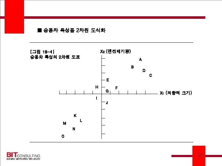

■ SPSS의 Quick Cluster → Classification cluster center를 계산하여 각 cluster의 평균을 계산하여 다시 입력자료로 사용하는 방법 [그림 18 -5] 단일결합방식 에 의한 결과 A D B C E G J F H I K M O L 1 2 3 4 5 6 N 7 8 9 10 11 12 13 14 12/3/2020 22

■ SPSS의 Quick Cluster → Classification cluster center를 계산하여 각 cluster의 평균을 계산하여 다시 입력자료로 사용하는 방법 [그림 18 -6] 완전결합방식 에 의한 결과 A D B C E G J F H I N M O L 1 2 3 5 K 4 6 6 7 9 11 10 12 13 14 12/3/2020 23
 Example 2 ■ 목적 : 회사 특성의 중요성 평가에 따른 고객 분류 (Stage")
(2) Example 2 ■ 목적 : 회사 특성의 중요성 평가에 따른 고객 분류 (Stage 1) Partitioning Step 1 : Hierarchical cluster Analysis 1) Similarity measure : Squared Euclidean distances 2) Algorithm : Ward's method ⇒ within-cluster difference를 최소화 3) cluster 수 결정 : Two cluster가 최선안으로 결정 12/3/2020 24
![TABLE 7. 2 Analysis of Agglomeration Coefficient for Hierarchical Cluster Analysis 12/3/2020 Number of]](http://slidetodoc.com/presentation_image_h/d957ca98c9afee004876f182c0a7d673/image-26.jpg "TABLE 7. 2 Analysis of Agglomeration Coefficient for Hierarchical Cluster Analysis 12/3/2020 Number of]")
TABLE 7. 2 Analysis of Agglomeration Coefficient for Hierarchical Cluster Analysis 12/3/2020 Number of] Clusters Percentage Change in Agglomeration Coefficient to Next Level 10 9 8 7 6 5 4 3 2 1 8. 9 8. 5 9. 2 9. 3 12. 1 17. 0 17. 6 61. 9 - 25

Step 2 : Nonhierarchical Cluster Analysis → hierarchical procedure 결과를 Fine-tune ⇒ Hierarchical procedure의 결과 확인 Results of Nonhierarchical Cluster Analysis with Initial Seed Points from Hierarchical Results Mean Values* Cluster X 1 X 2 X 3 X 4 X 5 X 6 X 7 1. 39 3. 22 8. 70 6. 74 5. 09 5. 69 2. 94 2. 87 2. 65 2. 87 5. 91 8. 10 1. 58 3. 21 8. 90 6. 80 4. 92 5. 60 2. 96 2. 87 2. 52 2. 82 5. 90 8. 13 Cluster Size Classification cluster centers 1 2 4. 40 2. 43 Final cluster centers 1 2 12/3/2020 4. 38 2. 57 52 48 26

Variables Cluster M. S. Df Error M. S df F Ratio Probability Significance Testing of Differences Between Cluster Centers X 1 X 2 X 3 X 4 X 5 X 6 X 7 Delivery speed Price level Price flexibility Manufacturer’s image Overall service Sales force’s image Product quality 81. 5631 66. 4571 109. 6372 11. 3023. 1883 2. 1233 123. 3719 1 1 1 1 . 9298. 7661. 8233 1. 1778. 5682. 5786 1. 2797 98. 0 98. 0 87. 7172 86. 7526 133. 1750 9. 5959. 3314 3. 6697 96. 4042 . 000. 003. 566. 058. 000 * X 1 = Delivery speed : X 2 = Price level : X 3 = Price flexibility : X 4 = Manufacturer’s image : X 5 = Overall service : X 6 = Sales force’s image : X 7 = Product quality. 12/3/2020 27

Group Means and Significance Level for Two-Group Nonhierarchical Cluster Solution Cluster Variables 1 2 F Ratio Significance 4. 460 1. 576 8. 900 4. 926 2. 992 2. 510 5. 904 2. 570 3. 152 6. 888 5. 570 2. 840 2. 820 8. 038 105. 00 76. 61 111. 30 8. 73 1. 02 4. 17 82. 68 . 0000. 0039. 3141. 0438. 0000 42. 32 4. 38 21. 312 26. 545 . 0000 Stage Two : Interpretation X 1 X 2 X 3 X 4 X 5 X 6 X 7 Delivery speed Price level Price flexibility Manufacturer’s image Overall service Sales force’s image Product quality Stage Three : Profiling Other variables of interest X 9 Usage level X 10 Satisfaction level 12/3/2020 49. 88 5. 16 28

Stage Two : Interpretation - Table 7. 4 참조 - X 5는 두 그룹 사이에 차이가 없는 것으로 평가됨 - Cluster 1 focuses ⅰ) delivery speed ⅱ) price flexibility Cluster 2 focuses ⅰ) price ⅱ) manufacturer's image ⅲ) sales force image ⅳ) product quality Stage Three : Validation - Table 7. 5 참조 (결과의 consistency 확인) ⇒ 무작위로 선택한 subset으로 clustering하여 비교 12/3/2020 29

TABLE 7. 5 Results of Nonhierarchical Cluster Analysis with Randomly Selected Initial Seed Points Cluster X 1 X 2 Classification cluster centers 1 4. 95 1. 14 2 1. 76 2. 70 Final cluster centers 1 4. 47 1. 57 2 2. 63 3. 10 X 3 Mean Values* X 4 X 5 X 6 X 7 Cluster Size 9. 03 6. 87 6. 55 5. 50 3. 21 1. 97 3. 79 2. 70 5. 09 8. 45 8. 93 6. 94 4. 99 5. 49 2. 99 2. 84 2. 57 2. 75 5. 78 8. 07 48 52 Significance Testing of Differences Between Cluster Centers Variables X 1 X 2 X 3 X 4 X 5 X 6 X 7 Cluster M. S. Delivery speed Price level Price flexibility Manufacturer’s image Overall service Sales force’s image Product quality 84. 3339 58. 6837 98. 5164 6. 2640. 5883. 7477 131. 1200 Df 1 1 1 1 Error M. S. 9016. 8454. 9367 1. 2292. 5641. 5927 1. 2007 df 98. 0 98. 0 F Value 93. 5415 69. 4175 105. 1700 5. 0958 1. 0428 1. 2616 109. 2055 Probability. 000. 026. 310. 264. 000 * X 1 = Delivery speed : X 2 = Price level : X 3 = Price flexibility : X 4 = Manufacturer’s image : X 5 = Overall service : X 6 = Sales force’s image : X 7 = Product quality. 12/3/2020 30
- Slides: 31