Cloud Computing Group 7 Advertising on the web

Cloud Computing Group 7

Advertising on the web • Sites such as e. Bay, OLX allow advertising for free or for charge • Companies like Amazon, Alibaba use ads to increase the sales • Ads placed on the search results • Factors that affect the advertisements Position of the ad -sports. yahoo. com/golf than yahoo homepage Query terms - apt to search queries
ONLINE – OFFLINE algorithms Matching of search queries to advertisements algorithms categorized OFFLINE • All the input data is available • Processed and made decision • Reliable and stable ONLINE • All input data is not available • On each stream decision needs to take place • Greedy approach • Not reliable but necessity
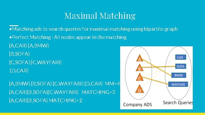
Maximal Matching • Matching ads to search queries for maximal matching using bipartite graph • Perfect Matching : All nodes appear in the matching {A, CAR} {A, BMW} {B, SOFA} {C, WAYFAIR} {D, CAR} MM=4 {A, CAR}{B, SOFA}{C, WAYFAIR} MATCHING=3 {A, CAR}{B, SOFA} MATCHING=2
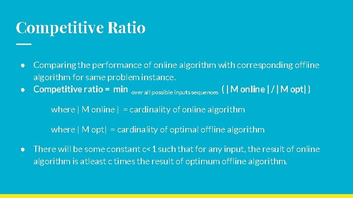
Competitive Ratio ● Comparing the performance of online algorithm with corresponding offline algorithm for same problem instance. ● Competitive ratio = min over all possible inputs sequences ( | M online | / | M opt| ) where | M online | = cardinality of online algorithm where | M opt| = cardinality of optimal offline algorithm ● There will be some constant c<1 such that for any input, the result of online algorithm is atleast c times the result of optimum offline algorithm.
Adwords ● ● ● Google’s Online Advertising Service Advertisers bid for queries on the search engine Search engine selects and displays ads for a small subset of the bidders Goal: Maximize search engine’s revenue Need for an online algorithm for maximizing revenue Metric used: AD RANK = CPC BID X QUALITY SCORE

Adwords Algorithm The Balance Algorithm ● Scenario: Advertisers: A and B; A bids on query x and B bids on queries x and y Sequence of queries: xxyy ● Query assigned to advertiser who has the maximum remaining budget ● Competitive Ratio = 3/4
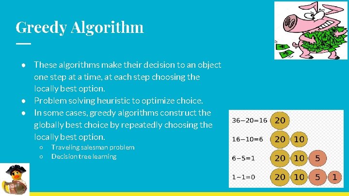
Greedy Algorithm ● These algorithms make their decision to an object one step at a time, at each step choosing the locally best option. ● Problem solving heuristic to optimize choice. ● In some cases, greedy algorithms construct the globally best choice by repeatedly choosing the locally best option. ○ ○ Traveling salesman problem Decision tree learning
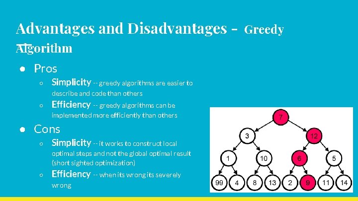
Advantages and Disadvantages Algorithm ● Pros ○ Simplicity -- greedy algorithms are easier to describe and code than others ○ Efficiency -- greedy algorithms can be implemented more efficiently than others ● Cons ○ Simplicity -- it works to construct local optimal steps and not the global optimal result (short sighted optimization) ○ Efficiency -- when its wrong its severely wrong Greedy
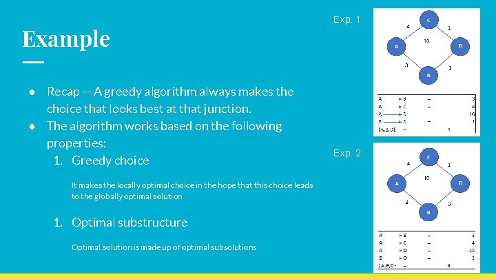
Example ● Recap -- A greedy algorithm always makes the choice that looks best at that junction. ● The algorithm works based on the following properties: 1. Greedy choice It makes the locally optimal choice in the hope that this choice leads to the globally optimal solution 1. Optimal substructure Optimal solution is made up of optimal subsolutions Exp. 1 Exp. 2
Performance-based advertising ● ● ● Introduced by Overture around the year 2000. Advertisers bid on keywords that we search in browser. Advertiser is charged only when there is an action on the link Google adopted this technique as “adwords”. Google observes CTR (click through rate), based on history Algorithms are developed to build keywords and ads to display for related keywords.
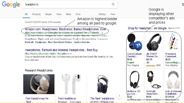
Amazon is highest bidder among all paid to google. Google is displaying other competitor’s ads and prices
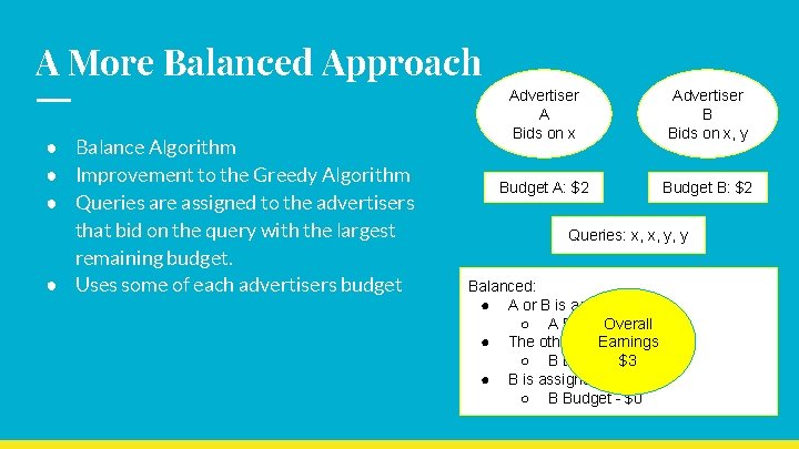
A More Balanced Approach ● Balance Algorithm ● Improvement to the Greedy Algorithm ● Queries are assigned to the advertisers that bid on the query with the largest remaining budget. ● Uses some of each advertisers budget Advertiser A Bids on x Advertiser B Bids on x, y Budget A: $2 Budget B: $2 Queries: x, x, y, y Greedy (Possible Outcome): Balanced: ● x ● B A is or assigned B is assigned x Overall ○ -- $1 ○ B A Budget. Overall $1 Earnings ● B is assigned x ● The other is assigned Earnings x ○ Budget - $2 $1 ○ B Budget -$3 $1 ● No Further Bids Available ● B is assigned y ○ B Budget - $0
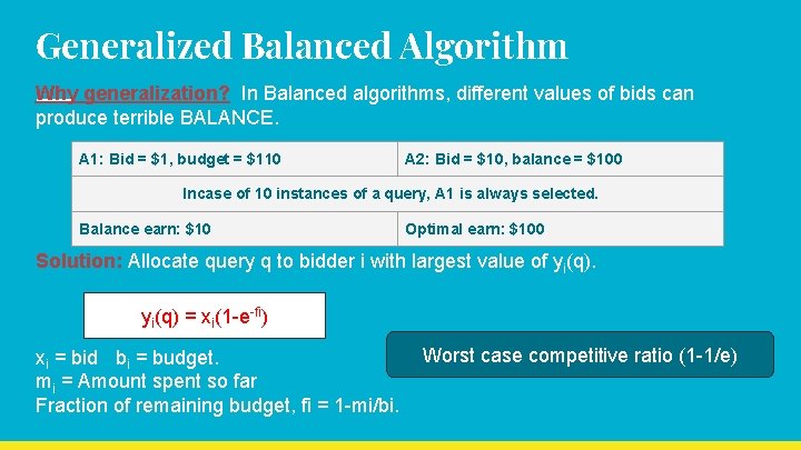
Generalized Balanced Algorithm Why generalization? In Balanced algorithms, different values of bids can produce terrible BALANCE. A 1: Bid = $1, budget = $110 A 2: Bid = $10, balance = $100 Incase of 10 instances of a query, A 1 is always selected. Balance earn: $10 Optimal earn: $100 Solution: Allocate query q to bidder i with largest value of yi(q) = xi(1 -e-fi) xi = bid bi = budget. mi = Amount spent so far Fraction of remaining budget, fi = 1 -mi/bi. Worst case competitive ratio (1 -1/e)
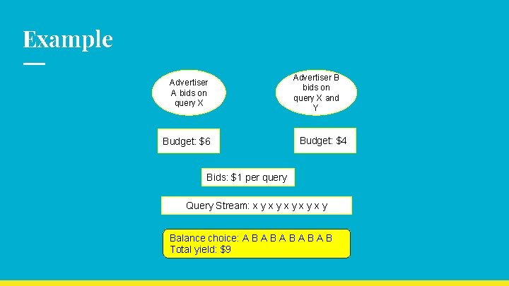
Example Advertiser A bids on query X Budget: $6 Advertiser B bids on query X and Y Budget: $4 Bids: $1 per query Query Stream: x y x y x y Balance choice: A B A B A B Total yield: $9
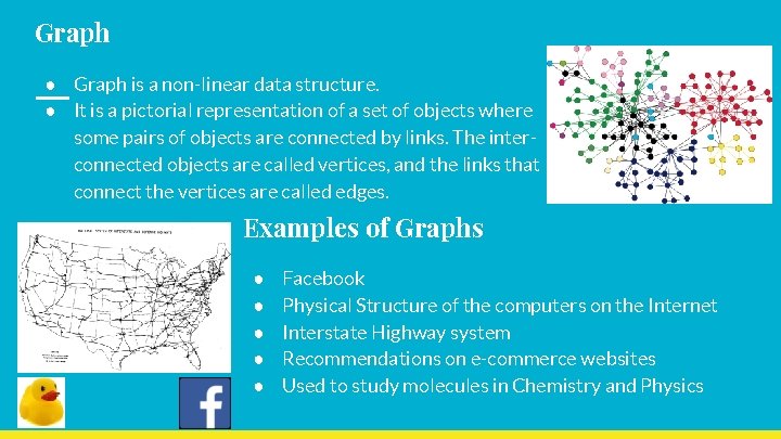
Graph ● Graph is a non-linear data structure. ● It is a pictorial representation of a set of objects where some pairs of objects are connected by links. The interconnected objects are called vertices, and the links that connect the vertices are called edges. Examples of Graphs ● ● ● Facebook Physical Structure of the computers on the Internet Interstate Highway system Recommendations on e-commerce websites Used to study molecules in Chemistry and Physics
Graph Problems ● Finding Shortest Path ○ Routing Internet Traffic and Logistics ● Finding Minimum Spanning Trees ○ Telephone Network Design ● Maximum Flow Problem ○ Airline Scheduling ● Bipartite Matching ○ Monster. com, Match. com ● Page. Rank Processing Graph Data ● As the size of the graph data is very large. Parallel processing has to be used for efficient computation. ● Techniques Used : Map. Reduce, Bulk-Synchronous Systems
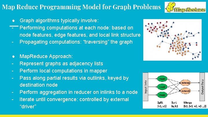
Map Reduce Programming Model for Graph Problems ● Graph algorithms typically involve: - Performing computations at each node: based on node features, edge features, and local link structure - Propagating computations: “traversing” the graph ● - Map. Reduce Approach: Represent graphs as adjacency lists Perform local computations in mapper Pass along partial results via outlinks, keyed by destination node Perform aggregation in reducer on inlinks to a node Iterate until convergence: controlled by external “driver”
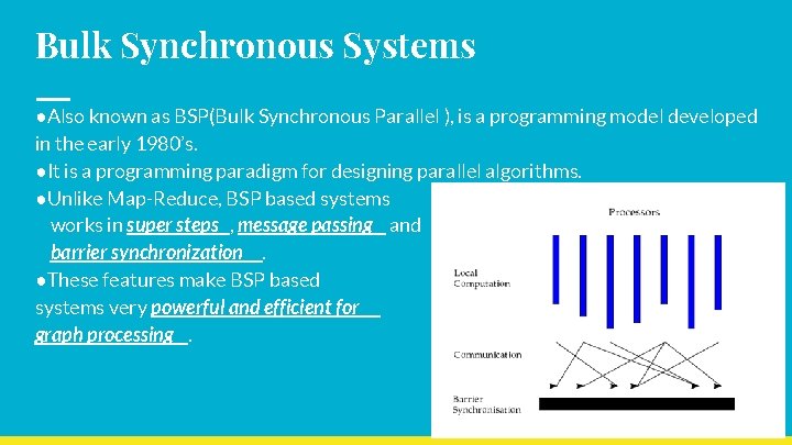
Bulk Synchronous Systems ●Also known as BSP(Bulk Synchronous Parallel ), is a programming model developed in the early 1980’s. ●It is a programming paradigm for designing parallel algorithms. ●Unlike Map-Reduce, BSP based systems works in super steps , message passing and barrier synchronization. ●These features make BSP based systems very powerful and efficient for graph processing.
Challenges in Graph Processing For most of the graph related algorithms, we face the following challenges ●Computation driven by data - algorithms execute based on the structure of graph, computation for each next vertex is strictly dependent on results calculated for all its ancestors. Partition is highly impossible. ●Diverse and unbalanced data structure skewed distribution of vertices degree. – graph is highly unstructured data with ●Data communication in comparison to computation
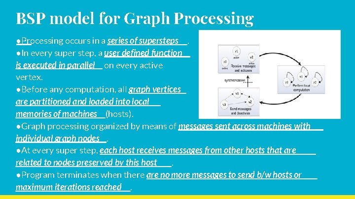
BSP model for Graph Processing ●Processing occurs in a series of supersteps. ●In every super step, a user defined function is executed in parallel on every active vertex. ●Before any computation, all graph vertices are partitioned and loaded into local memories of machines (hosts). ●Graph processing organized by means of messages sent across machines with individual graph nodes. ●At every super step, each host receives messages from other hosts that are related to nodes preserved by this host. ●Program terminates when there are no more messages to send b/w hosts or maximum iterations reached.

- Slides: 22