Cloud Computing Cloud Resource Allocation Issues Dept of

Cloud Computing: Cloud Resource Allocation Issues Dept. of Computer Science and Information Engineering National Central University 1 *Some slides are adopted from “Distributed and Cloud Computing from Parallel Processing to the Internet of Things” by K. Hwang, G. C. Fox and J. J. Dongarra

Outline Cloud Resource Allocation and Scheduling Overview of Iaa. S Scheduling Overview of Paa. S/Saa. S Scheduling 2

Cloud Resource Allocation Overview 3

Overview of Cloud Resource Allocation and Scheduling 4

Resource Allocation and Scheduling Resource allocation: an approach/mechanism to allocate resources to tasks/users Scheduling: 5 Scheduling is the approach/mechanism to find a schedule for all the resources that can serve all the tasks, given a set of resources and a set of tasks. A task may have dependency on other tasks

Computer Resource Allocation and Scheduling Critical function of any man-made system. It affects the three basic criteria for measuring system performance: Scheduling in a computing system deciding how to allocate resources of a system, such as CPU cycles, memory, secondary storage space, I/O and network bandwidth, between users and tasks. Policies and mechanisms for resource allocation. 6 Functionality. Performance. Cost. Policy principles guiding decisions. Mechanisms the means to implement policies.

Resource Allocation and Scheduling on the Cloud It cannot violate cloud management policies This kind of problem is usually hard: 7 Multi-objective optimization under complex policies and constraints Impossible to get accurate global state information. Affected by unpredictable events (e. g. system failures, attacks). Cloud service providers are faced with large fluctuating workloads/demands. The strategies for Iaa. S, Paa. S, and Saa. S are different.

Cloud Resource Management (CRM) Policies 1. Admission control prevent the system from accepting workload in violation of high-level system policies. 2. Capacity allocation allocate resources for individual activations of a service. 3. Load balancing distribute the workload evenly among the servers. 4. Energy optimization minimization of energy consumption. 5. Quality of service (Qo. S) guarantees ability to satisfy timing or other conditions specified by a Service Level Agreement. 8

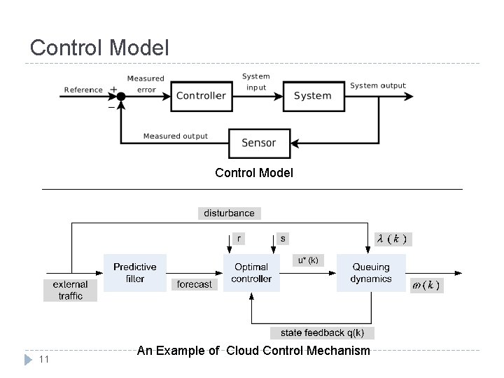
Mechanisms for the Implementation of Resource Management Policies Control theory uses the feedback to guarantee system stability and predict transient behavior. Machine learning does not need a performance model of the system. Utility-based require a performance model and a mechanism to correlate user-level performance with cost. Market-oriented/economic do not require a model of the system, e. g. , combinatorial auctions for bundles of resources. 9

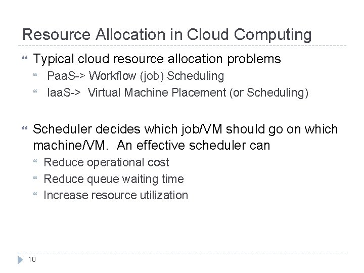
Resource Allocation in Cloud Computing Typical cloud resource allocation problems Paa. S-> Workflow (job) Scheduling Iaa. S-> Virtual Machine Placement (or Scheduling) Scheduler decides which job/VM should go on which machine/VM. An effective scheduler can 10 Reduce operational cost Reduce queue waiting time Increase resource utilization

Control Model 11 An Example of Cloud Control Mechanism

Overview of Iaa. S Resource Allocation 12

Overview of Iaa. S Resource Allocation Static VM Placement 13

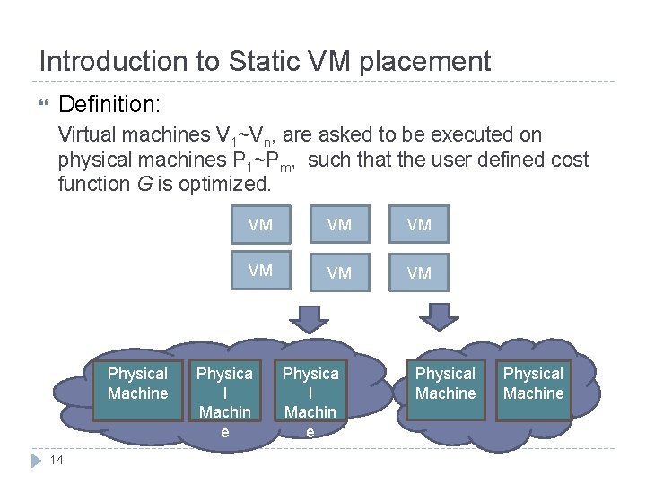
Introduction to Static VM placement Definition: Virtual machines V 1~Vn, are asked to be executed on physical machines P 1~Pm, such that the user defined cost function G is optimized. Physical Machine 14 VM VM VM Physica l Machin e Physical Machine

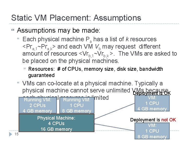
Static VM Placement: Assumptions may be made: Each physical machine Pa has a list of k resources <Pra, 1~Pra, k> and each VM Vb may request different amount of resources <Vrb, 1~Vrb, k >. The VMs are asked to be placed on the physical machines. Resources: # of CPUs, memory size, disk size, bandwidth guaranteed VMs can co-locate at a physical machine. Typically a physical machine cannot serve unlimited VMs because Deployment is OK VM: each physical resource is limited Running VM: 2 CPUs 1 CPU 4 GB memory 8 GB memory Physical Machine: 4 CPUs 16 GB memory 15 1 CPU 4 GB memory Deployment is not OK VM: 1 CPU 8 GB memory

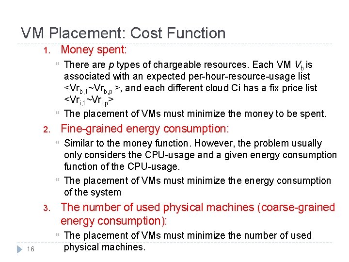
VM Placement: Cost Function Money spent: 1. Fine-grained energy consumption: 2. Similar to the money function. However, the problem usually only considers the CPU-usage and a given energy consumption function of the CPU-usage. The placement of VMs must minimize the energy consumption of the system The number of used physical machines (coarse-grained energy consumption): 3. 16 There are p types of chargeable resources. Each VM Vb is associated with an expected per-hour-resource-usage list <Vrb, 1~Vrb, p >, and each different cloud Ci has a fix price list <Vri, 1~Vri, p> The placement of VMs must minimize the money to be spent. The placement of VMs must minimize the number of used physical machines.

VM Placement: Cost Function (Cont. ) Load balancing: 4. Multi-objective optimization: 5. 17 The placement makes a similar workload of each physical host Try to optimize several goals at a time.

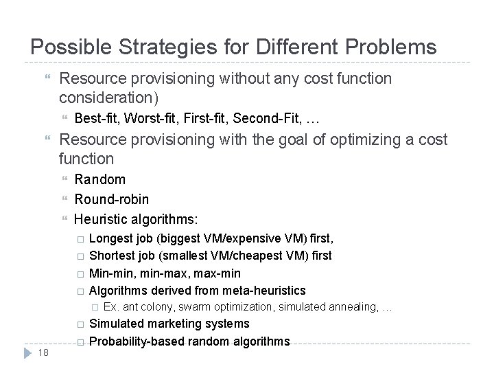
Possible Strategies for Different Problems Resource provisioning without any cost function consideration) Best-fit, Worst-fit, First-fit, Second-Fit, … Resource provisioning with the goal of optimizing a cost function Random Round-robin Heuristic algorithms: Longest job (biggest VM/expensive VM) first, Shortest job (smallest VM/cheapest VM) first Min-min, min-max, max-min Algorithms derived from meta-heuristics 18 Ex. ant colony, swarm optimization, simulated annealing, … Simulated marketing systems Probability-based random algorithms

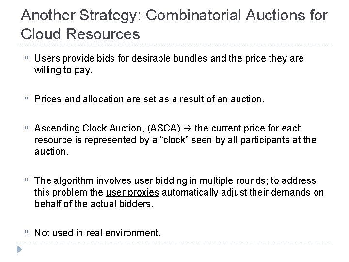
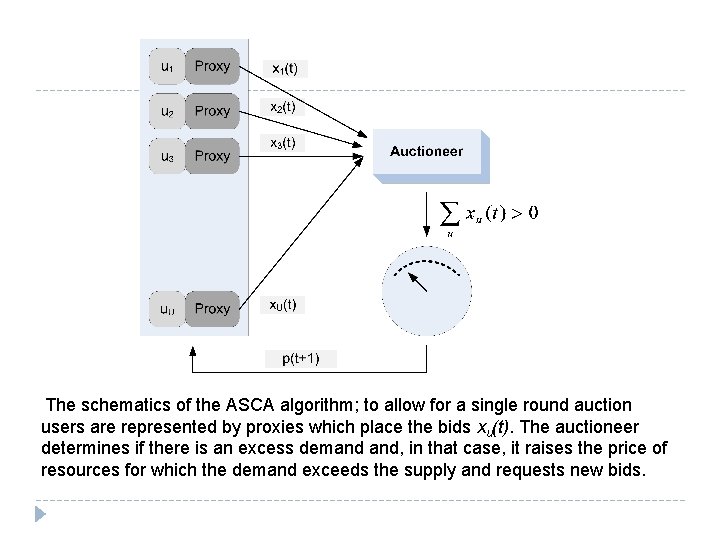
Another Strategy: Combinatorial Auctions for Cloud Resources Users provide bids for desirable bundles and the price they are willing to pay. Prices and allocation are set as a result of an auction. Ascending Clock Auction, (ASCA) the current price for each resource is represented by a “clock” seen by all participants at the auction. The algorithm involves user bidding in multiple rounds; to address this problem the user proxies automatically adjust their demands on behalf of the actual bidders. Not used in real environment.

The schematics of the ASCA algorithm; to allow for a single round auction users are represented by proxies which place the bids xu(t). The auctioneer determines if there is an excess demand and, in that case, it raises the price of resources for which the demand exceeds the supply and requests new bids.

Overview of Iaa. S Resource Allocation Dynamic VM Placement 21

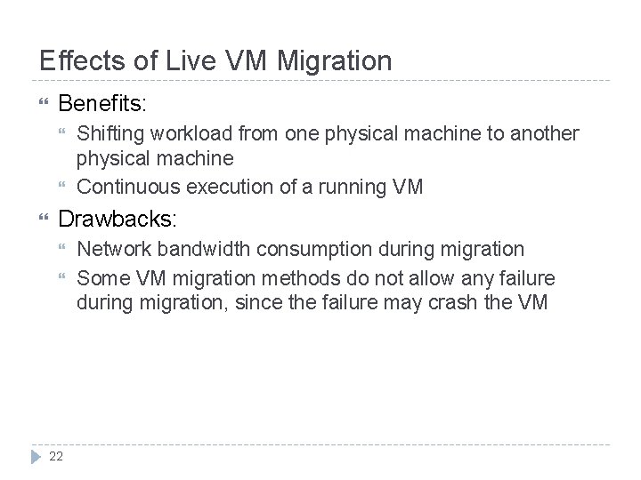
Effects of Live VM Migration Benefits: Shifting workload from one physical machine to another physical machine Continuous execution of a running VM Drawbacks: 22 Network bandwidth consumption during migration Some VM migration methods do not allow any failure during migration, since the failure may crash the VM

Dynamic VM Placement Dynamic VM placement: Use VM migration to reconfigure the cloud system periodically Migration may introduce overheads Possible Goal: Re-optimize the cost function (used in static VM placement) Disaster prevention 23 The assumption is that resource usage of a VM is a time function. So reconfiguration may have benefits Example case: a physical machine has been detected an abnormal working temperature. We can migrate the VM to another physical machine in advance since the abnormal physical machine may crash at any time. When to do reconfiguration: Periodically Event-driven

Overview of Iaa. S Resource Allocation Auto-Scaling 24

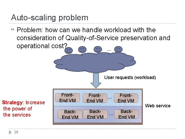
Auto-scaling problem Problem: how can we handle workload with the consideration of Quality-of-Service preservation and operational cost? … User requests (workload) Strategy: Increase the power of the services 25 Front. End VM Back. End VM Front- … End VM Front. End VM Back. End VM … Web service

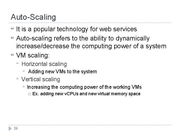
Auto-Scaling It is a popular technology for web services Auto-scaling refers to the ability to dynamically increase/decrease the computing power of a system VM scaling: Horizontal scaling Adding new VMs to the system Vertical scaling Increasing the computing power of the working VMs 26 Ex. adding new v. CPUs and new virtual memory space

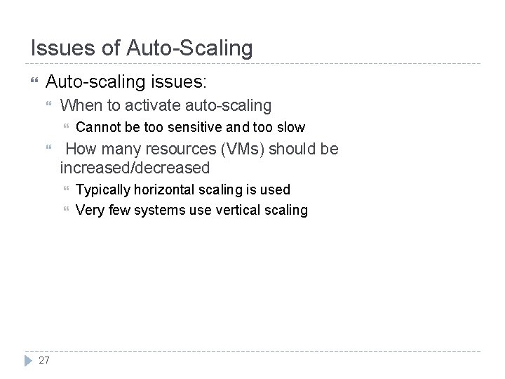
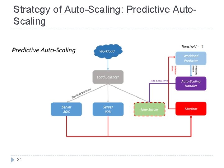
Issues of Auto-Scaling Auto-scaling issues: When to activate auto-scaling How many resources (VMs) should be increased/decreased 27 Cannot be too sensitive and too slow Typically horizontal scaling is used Very few systems use vertical scaling

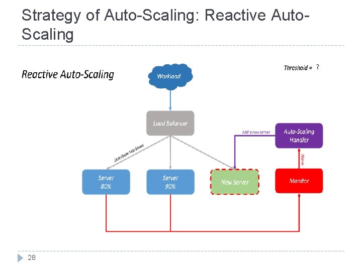
Strategy of Auto-Scaling: Reactive Auto. Scaling 28

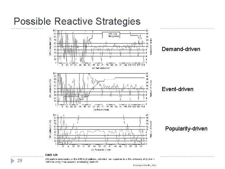
Possible Reactive Strategies Demand-driven Event-driven Popularity-driven 29

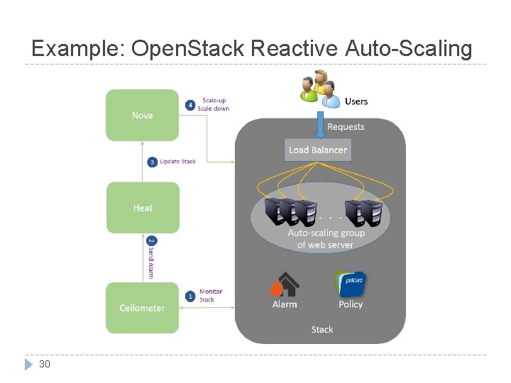
Example: Open. Stack Reactive Auto-Scaling 30

Strategy of Auto-Scaling: Predictive Auto. Scaling 31

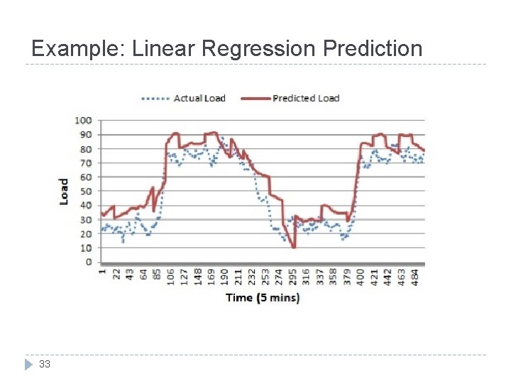
Possible Predictive Strategies They can predict the resources that will be used Prediction workload Linear regression calculation [1] Using Chaos Theory to predict [2] Auto-regressive model[3] Bayesian Network with machine learning techniques[4] [1] K. Qazi, Yang Li, and A. Sohn, “Workload Prediction of Virtual Machines for Harnessing Data Center Resources, ”in 2014 IEEE 7 th International Conference on Cloud Computing (CLOUD), 2014, pp. 522– 529. [2] L. Yazdanov and C. Fetzer, “Lightweight automatic resource scaling for multi-tier web applications, ” in 2014 IEEE 7 th International Conference on Cloud Computing (CLOUD), 2014, pp. 466– 473 [3] A. Bashar, “Autonomic scaling of Cloud Computing resources using BN-based prediction models, ” in 2013 IEEE 2 nd International Conference on Cloud Networking (Cloud. Net), 2013, pp. 200– 204 [4] L. Zhang, Y. Zhang, P. Jamshidi, L. Xu, and C. Pahl, “Workload Patterns for Quality-Driven Dynamic Cloud Service Configuration and Auto-Scaling, ” in Proceedings of the 2014 IEEE/ACM 7 th International Conference on Utility and Cloud Computing, 2014, pp. 156– 165. 32

Example: Linear Regression Prediction 33

Comparison of Reactive and Predictive Strategies Reactive auto-scaling: Tell the system when to do auto-scaling Predictive auto-scaling: 34 In most studies, it tells the system how to do auto-scaling Studies for temporal prediction are very few

Overview of Iaa. S Resource Allocation Choice: Private cloud or public cloud 35

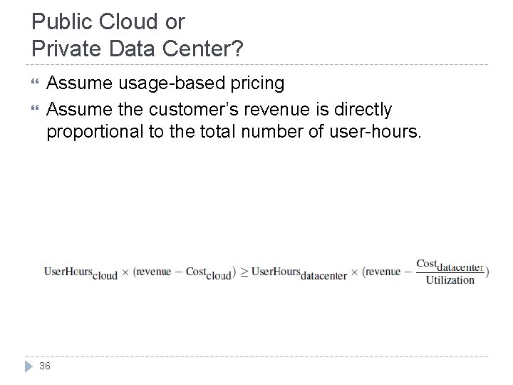
Public Cloud or Private Data Center? Assume usage-based pricing Assume the customer’s revenue is directly proportional to the total number of user-hours. 36

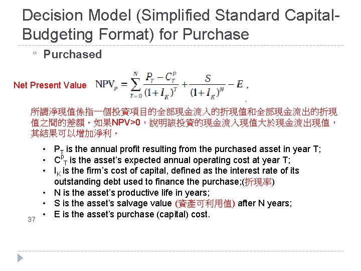
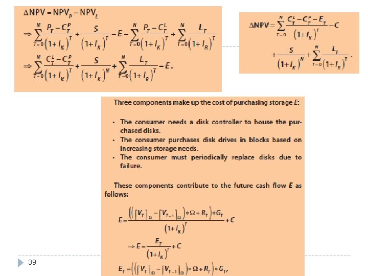
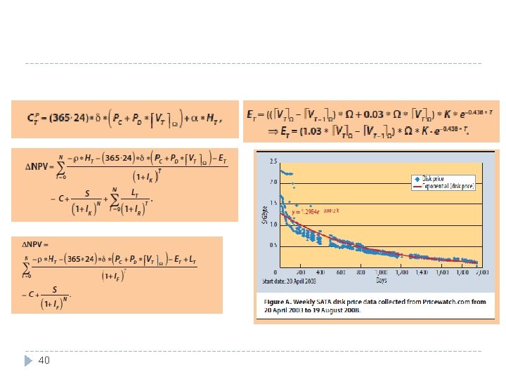
Decision Model (Simplified Standard Capital. Budgeting Format) for Purchased Net Present Value 所謂淨現值係指一個投資項目的全部現金流入的折現值和全部現金流出的折現 值之間的差額。如果NPV>0，說明該投資的現金流入現值大於現金流出現值， 其結果可以增加淨利。 37 • PT is the annual profit resulting from the purchased asset in year T; • Cp. T is the asset’s expected annual operating cost at year T; • IK is the firm’s cost of capital, defined as the interest rate of its outstanding debt used to finance the purchase; (折現率) • N is the asset’s productive life in years; • S is the asset’s salvage value (資產可利用值) after N years; • E is the asset’s purchase (capital) cost.

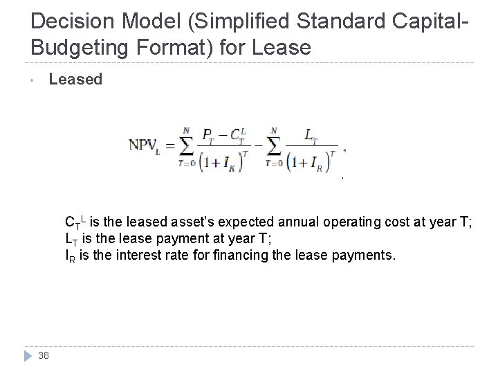
Decision Model (Simplified Standard Capital. Budgeting Format) for Lease • Leased CTL is the leased asset’s expected annual operating cost at year T; LT is the lease payment at year T; IR is the interest rate for financing the lease payments. 38

39

40

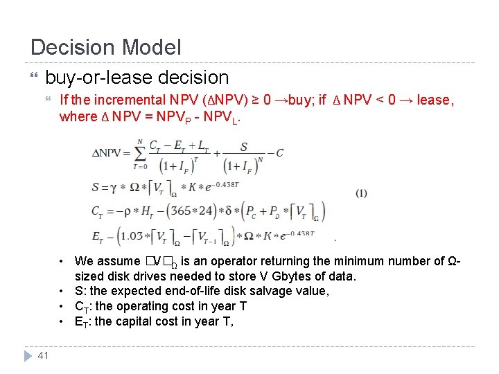
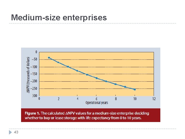
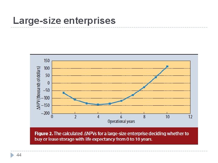
Decision Model buy-or-lease decision If the incremental NPV (ΔNPV) ≥ 0 →buy; if Δ NPV < 0 → lease, where Δ NPV = NPVP - NPVL. • We assume �V�Ω is an operator returning the minimum number of Ωsized disk drives needed to store V Gbytes of data. • S: the expected end-of-life disk salvage value, • CT: the operating cost in year T • ET: the capital cost in year T, 41

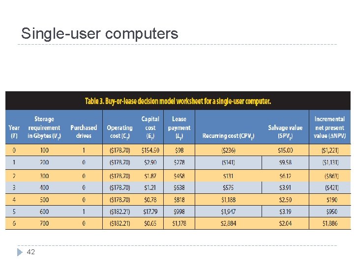
Single-user computers 42

Medium-size enterprises 43

Large-size enterprises 44

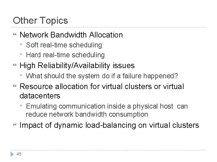
Other Topics Network Bandwidth Allocation High Reliability/Availability issues What should the system do if a failure happened? Resource allocation for virtual clusters or virtual datacenters Soft real-time scheduling Hard real-time scheduling Emulating communication inside a physical host can reduce network bandwidth consumption Impact of dynamic load-balancing on virtual clusters 45

Overview of Paa. S/Saa. S Resource Allocation 46

Overview of Paa. S/Saa. S Resource Allocation Concept of Paa. S/Saa. S Scheduling 47

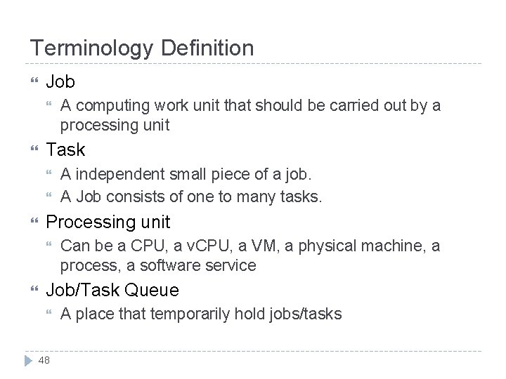
Terminology Definition Job Task A independent small piece of a job. A Job consists of one to many tasks. Processing unit A computing work unit that should be carried out by a processing unit Can be a CPU, a v. CPU, a VM, a physical machine, a process, a software service Job/Task Queue 48 A place that temporarily hold jobs/tasks

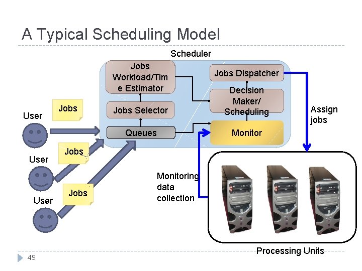
A Typical Scheduling Model Scheduler Jobs Workload/Tim e Estimator User 49 Jobs Dispatcher Jobs Selector Decision Maker/ Scheduling Queues Monitor Assign jobs Jobs Monitoring data collection Processing Units

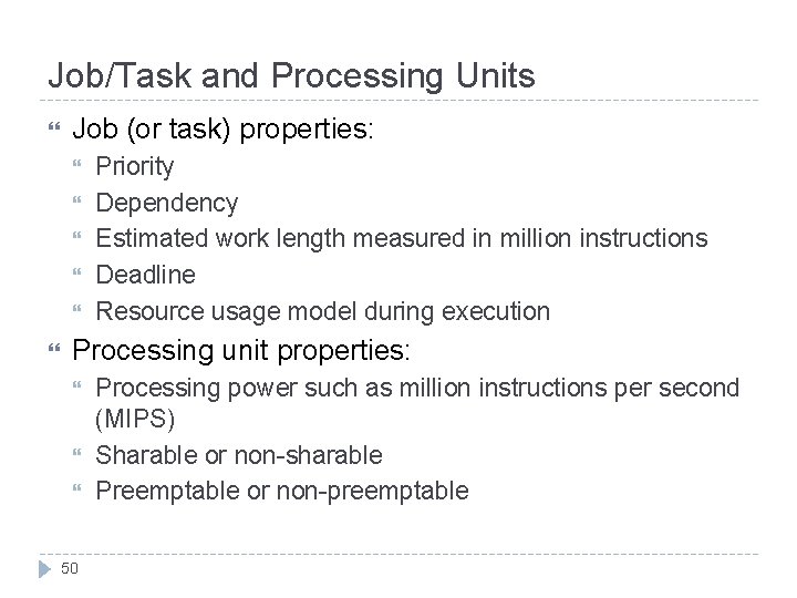
Job/Task and Processing Units Job (or task) properties: Priority Dependency Estimated work length measured in million instructions Deadline Resource usage model during execution Processing unit properties: 50 Processing power such as million instructions per second (MIPS) Sharable or non-sharable Preemptable or non-preemptable

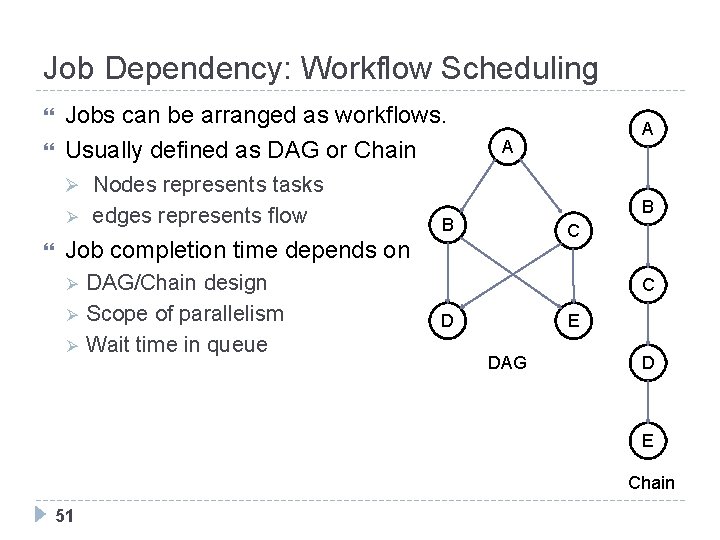
Job Dependency: Workflow Scheduling Jobs can be arranged as workflows. Usually defined as DAG or Chain A A Ø Nodes represents tasks Ø edges represents flow B B C Job completion time depends on Ø Ø Ø DAG/Chain design Scope of parallelism Wait time in queue C D E DAG D E Chain 51

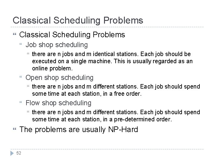
Classical Scheduling Problems Job shop scheduling Open shop scheduling there are n jobs and m different stations. Each job should spend some time at each station, in a free order. Flow shop scheduling there are n jobs and m identical stations. Each job should be executed on a single machine. This is usually regarded as an online problem. there are n jobs and m different stations. Each job should spend some time at each station, in a pre-determined order. The problems are usually NP-Hard 52

Job/Task Scheduling on Clouds Most scheduling problems on the clouds belong to Job shop scheduling Job scheduling means to place jobs to a set of processing units for execution Task scheduling has a similar definition Assume we are given a set of jobs to be executed and a set of processing units: 53 A job scheduler should calculate “a schedule” for each job describing when the job is started on which processing unit It must ensure no rules (constraints) are broken It may need to calculate the “cost” of the schedule, given a cost function (such as a pricing model on an open cloud)

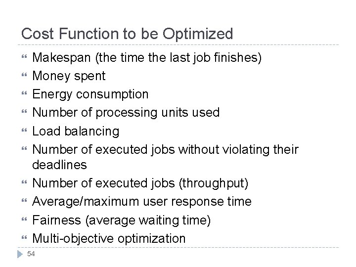
Cost Function to be Optimized Makespan (the time the last job finishes) Money spent Energy consumption Number of processing units used Load balancing Number of executed jobs without violating their deadlines Number of executed jobs (throughput) Average/maximum user response time Fairness (average waiting time) Multi-objective optimization 54

Overview of Paa. S/Saa. S Resource Allocation Scheduling Strategies 55

Preconditions of Scheduling The work length (in million instructions) of a job can or cannot be estimated The pool of processing units is homogeneous or heterogeneous The specific scheduling constraints 56 Failure rate of processing unit Price of using the processing units …

Scheduling Methods for Unknown Work Length with Homogeneous Environment Round-Robin Random High-Priority-First 57

Scheduling Methods for Estimable Work Length with Homogeneous Environment Shortest-task-first Longest-task-first Round-Robin Random High-Priority-First 58

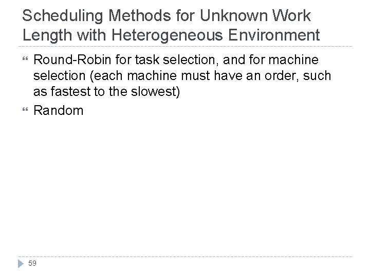
Scheduling Methods for Unknown Work Length with Heterogeneous Environment Round-Robin for task selection, and for machine selection (each machine must have an order, such as fastest to the slowest) Random 59

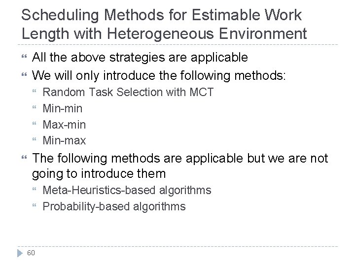
Scheduling Methods for Estimable Work Length with Heterogeneous Environment All the above strategies are applicable We will only introduce the following methods: Random Task Selection with MCT Min-min Max-min Min-max The following methods are applicable but we are not going to introduce them 60 Meta-Heuristics-based algorithms Probability-based algorithms

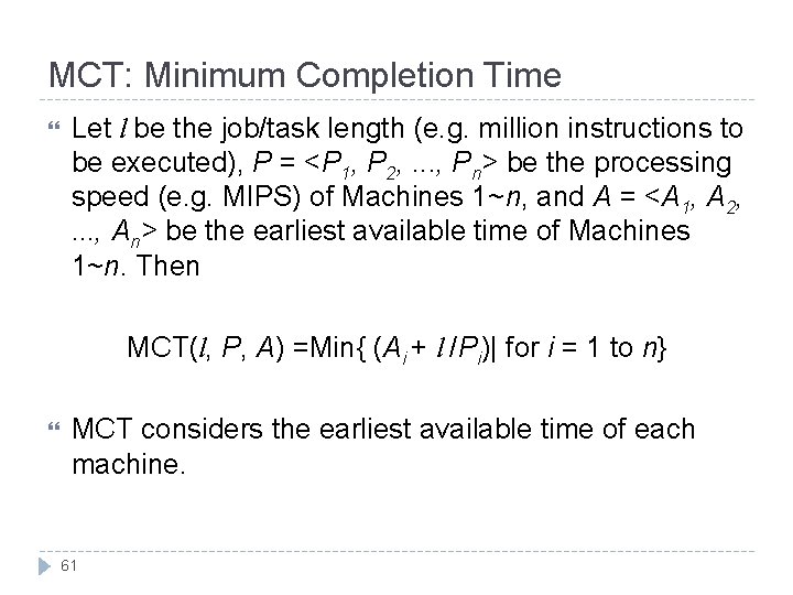
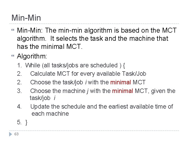
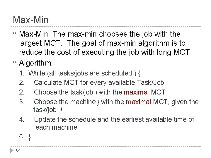
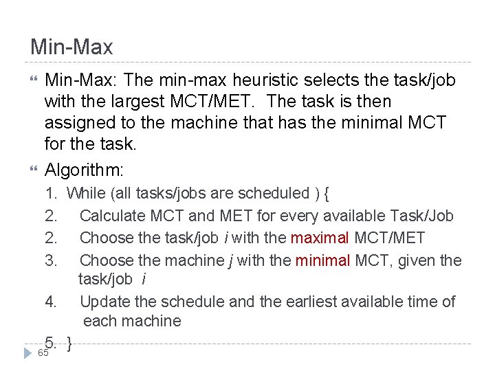
MCT: Minimum Completion Time Let l be the job/task length (e. g. million instructions to be executed), P = <P 1, P 2, . . . , Pn> be the processing speed (e. g. MIPS) of Machines 1~n, and A = <A 1, A 2, . . . , An> be the earliest available time of Machines 1~n. Then MCT(l, P, A) =Min{ (Ai + l /Pi)| for i = 1 to n} MCT considers the earliest available time of each machine. 61

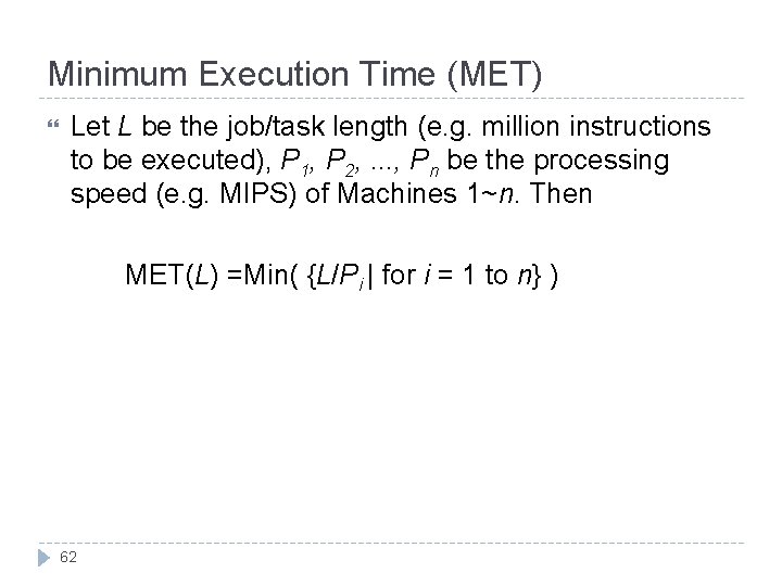
Minimum Execution Time (MET) Let L be the job/task length (e. g. million instructions to be executed), P 1, P 2, . . . , Pn be the processing speed (e. g. MIPS) of Machines 1~n. Then MET(L) =Min( {L/Pi | for i = 1 to n} ) 62

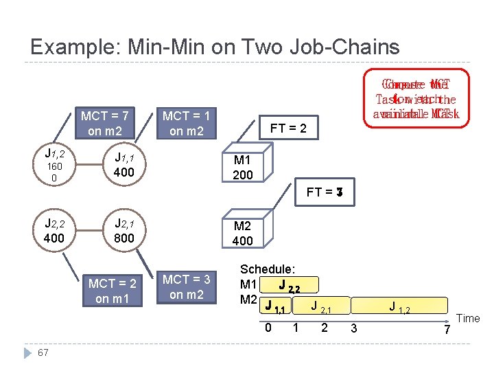
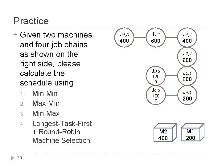
Min-Min Min-Min: The min-min algorithm is based on the MCT algorithm. It selects the task and the machine that has the minimal MCT. Algorithm: 1. While (all tasks/jobs are scheduled ) { 2. Calculate MCT for every available Task/Job 2. Choose the task/job i with the minimal MCT 3. Choose the machine j with the minimal MCT, given the task/job i 4. Update the schedule and the earliest available time of each machine 5. } 63

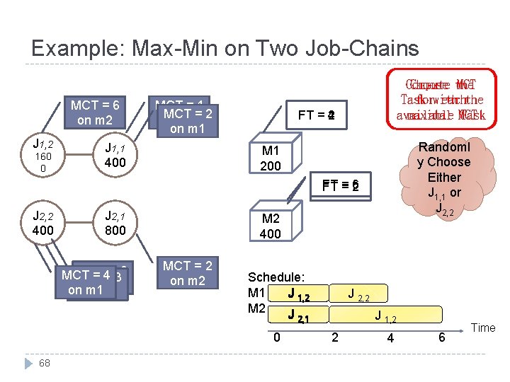
Max-Min Max-Min: The max-min chooses the job with the largest MCT. The goal of max-min algorithm is to reduce the cost of executing the job with long MCT. Algorithm: 1. While (all tasks/jobs are scheduled ) { 2. Calculate MCT for every available Task/Job 2. Choose the task/job i with the maximal MCT 3. Choose the machine j with the maximal MCT, given the task/job i 4. Update the schedule and the earliest available time of each machine 5. } 64

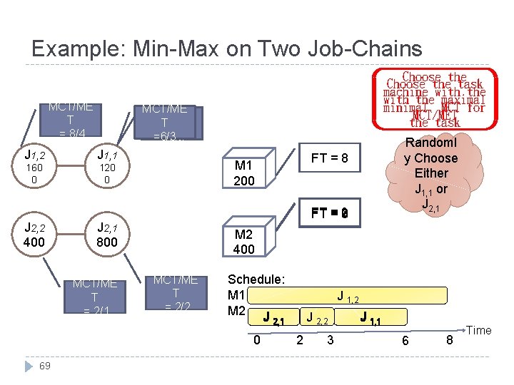
Min-Max Min-Max: The min-max heuristic selects the task/job with the largest MCT/MET. The task is then assigned to the machine that has the minimal MCT for the task. Algorithm: 1. While (all tasks/jobs are scheduled ) { 2. Calculate MCT and MET for every available Task/Job 2. Choose the task/job i with the maximal MCT/MET 3. Choose the machine j with the minimal MCT, given the task/job i 4. Update the schedule and the earliest available time of each machine 5. } 65

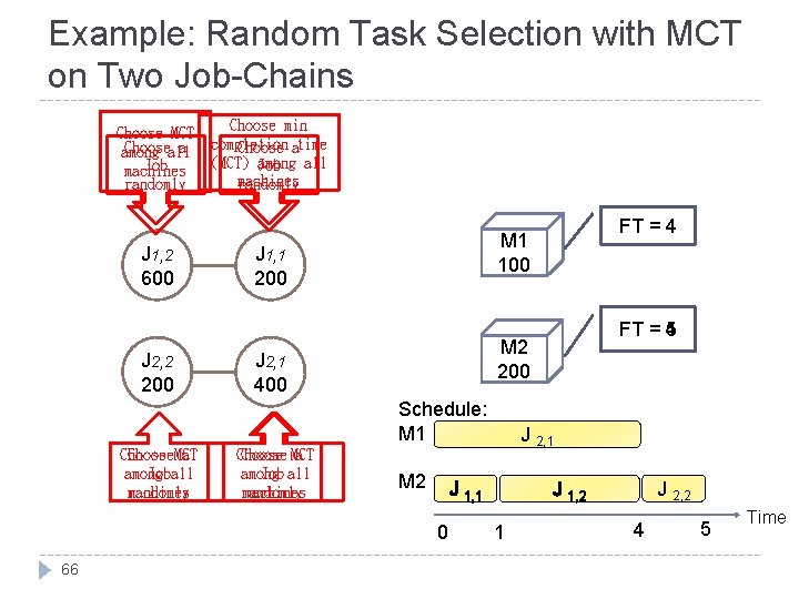
Example: Random Task Selection with MCT on Two Job-Chains Choose MCT Chooseall a among Job machines randomly J 1, 2 600 J 2, 2 200 Choose min completion Choose atime (MCT) among Job all machines randomly J 1, 1 200 Choose MCT a among Job all randomly machines M 2 J 2, 1 J 1, 1 0 66 FT = 4 1 5 M 2 200 J 2, 1 400 Schedule: M 1 Choose. MCT a among Joball randomly machines FT = 4 M 1 100 J 2, 2 J 1, 2 1 4 5 Time

Example: Min-Min on Two Job-Chains MCT = 7 5 on m 2 J 1, 2 160 0 Compute MCT Choose the forwith eachthe Task available Task minimal MCT = 1 on m 2 J 1, 1 400 FT = 2 M 1 200 FT = 3 1 7 J 2, 2 400 J 2, 1 800 MCT = 2 on m 1 M 2 400 MCT = 3 2 on m 2 Schedule: M 1 J 2, 2 M 2 J 1, 1 J 2, 1 0 67 1 2 J 1, 2 3 7 Time

Example: Max-Min on Two Job-Chains MCT = 6 on m 2 J 1, 2 160 0 MCT = 1 MCT = 2 on m 1 J 1, 1 400 Compute Choose the MCT Task forwith eachthe available maximal MCT Task FT = 4 2 Randoml y Choose Either J 1, 1 or J 2, 2 M 1 200 FT = 6 2 J 2, 2 400 J 2, 1 800 MCT =2 MCT =4 MCT =3 on m 1 onon m 1 m 2 M 2 400 MCT = 2 on m 2 Schedule: M 1 J 1, 2 M 2 J 2, 1 0 68 J 2, 2 J 1, 2 2 4 6 Time

Example: Min-Max on Two Job-Chains MCT/ME T = 8/4 MCT/ME TT =6/3 == 5/3 3/3 J 1, 2 J 1, 1 160 0 120 0 J 2, 2 400 Choose the task machine with the maximal minimal MCT for MCT/MET the task 3 2 FT = 6 M 2 400 MCT/ME T = 2/2 Schedule: M 1 M 2 J 2, 1 0 69 FT = 8 M 1 200 J 2, 1 800 MCT/ME T = 2/1 Randoml y Choose Either J 1, 1 or J 2, 1 J 1, 2 J 2, 2 2 3 J 1, 1 6 8 Time

Practice Given two machines and four job chains as shown on the right side, please calculate the schedule using 1. 2. 3. 4. 70 Min-Min Max-Min Min-Max Longest-Task-First + Round-Robin Machine Selection J 1, 3 400 J 1, 2 600 J 1, 1 400 J 2, 1 600 J 3, 2 120 0 J 4, 2 100 0 M 2 400 J 3, 1 800 J 4, 1 200 M 1 200