Closures of Relations Transitive Closure and Partitions Sections

Closures of Relations: Transitive Closure and Partitions Sections 8. 4 and 8. 5 1

Concept of “closure” n n The natural numbers N (counting numbers) are not closed under subtraction: when we close them under subtraction, we get Z, the integers (positive and negative). When we close Z under the operation of division, we get Q, the rational numbers. “Closing” a relation has important applications.

Transitive closure Computing the transitive closure of a digraph is an important problem in many computer science applications: n q q q Evaluation of recursive database queries. Analysis of reachability (connectivity) of transition graphs in communication networks. Construction of parsing automata in compilers. 3

Introduction Closure of relation properties n q When a property does not hold for a relation, how could we minimally augment the relation so that the property would hold? 4

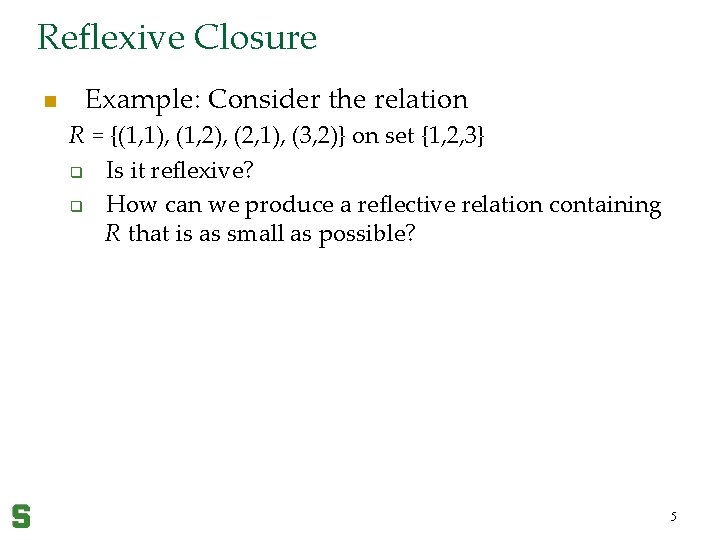
Reflexive Closure n Example: Consider the relation R = {(1, 1), (1, 2), (2, 1), (3, 2)} on set {1, 2, 3} q Is it reflexive? q How can we produce a reflective relation containing R that is as small as possible? 5

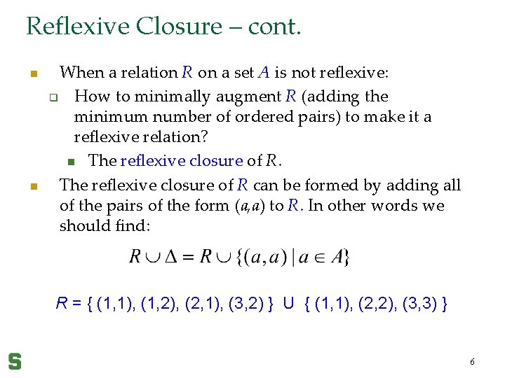
Reflexive Closure – cont. n n When a relation R on a set A is not reflexive: q How to minimally augment R (adding the minimum number of ordered pairs) to make it a reflexive relation? n The reflexive closure of R can be formed by adding all of the pairs of the form (a, a) to R. In other words we should find: R = { (1, 1), (1, 2), (2, 1), (3, 2) } U { (1, 1), (2, 2), (3, 3) } 6

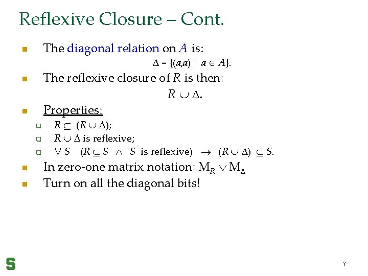
Reflexive Closure – Cont. The diagonal relation on A is: n = {(a, a) | a A}. The reflexive closure of R is then: R . Properties: n n q q q n n R (R ); R is reflexive; S (R S S is reflexive) (R ) S. In zero-one matrix notation: MR M Turn on all the diagonal bits! 7

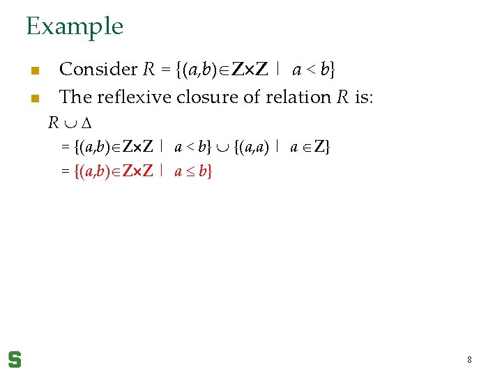
Example n n Consider R = {(a, b) Z Z | a < b} The reflexive closure of relation R is: R = {(a, b) Z Z | a < b} {(a, a) | a Z} = {(a, b) Z Z | a b} 8

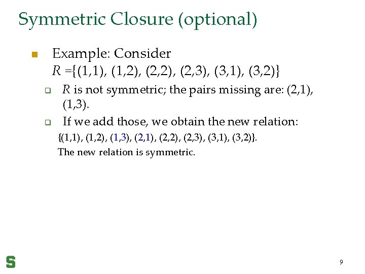
Symmetric Closure (optional) Example: Consider R ={(1, 1), (1, 2), (2, 3), (3, 1), (3, 2)} n q q R is not symmetric; the pairs missing are: (2, 1), (1, 3). If we add those, we obtain the new relation: {(1, 1), (1, 2), (1, 3), (2, 1), (2, 2), (2, 3), (3, 1), (3, 2)}. The new relation is symmetric. 9

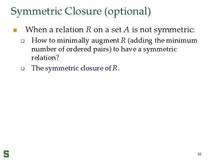
Symmetric Closure (optional) When a relation R on a set A is not symmetric: n q q How to minimally augment R (adding the minimum number of ordered pairs) to have a symmetric relation? The symmetric closure of R. 10

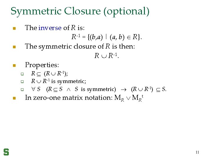
Symmetric Closure (optional) The inverse of R is: R-1 = {(b, a) | (a, b) R}. The symmetric closure of R is then: R R-1. Properties: n n n q q q n R (R R-1); R R-1 is symmetric; S (R S S is symmetric) (R R-1) S. In zero-one matrix notation: MR MRt 11

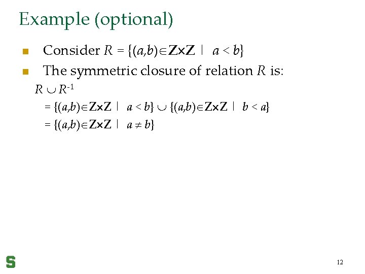
Example (optional) n n Consider R = {(a, b) Z Z | a < b} The symmetric closure of relation R is: R R-1 = {(a, b) Z Z | a < b} {(a, b) Z Z | b < a} = {(a, b) Z Z | a b} 12

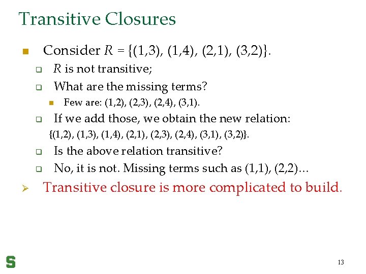
Transitive Closures Consider R = {(1, 3), (1, 4), (2, 1), (3, 2)}. n R is not transitive; What are the missing terms? q q n q Few are: (1, 2), (2, 3), (2, 4), (3, 1). If we add those, we obtain the new relation: {(1, 2), (1, 3), (1, 4), (2, 1), (2, 3), (2, 4), (3, 1), (3, 2)}. q q Ø Is the above relation transitive? No, it is not. Missing terms such as (1, 1), (2, 2)… Transitive closure is more complicated to build. 13

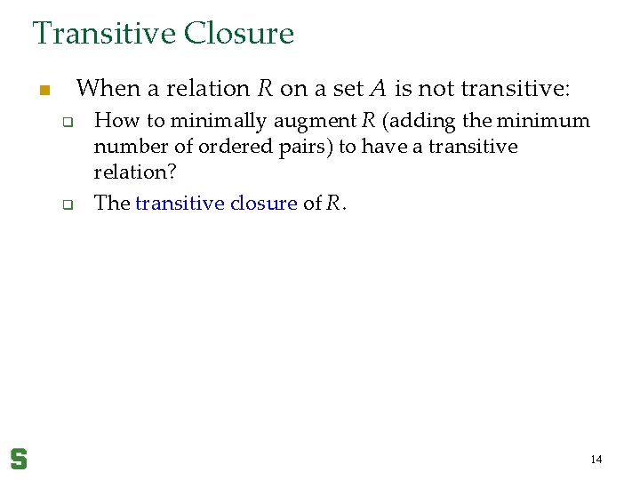
Transitive Closure When a relation R on a set A is not transitive: n q q How to minimally augment R (adding the minimum number of ordered pairs) to have a transitive relation? The transitive closure of R. 14

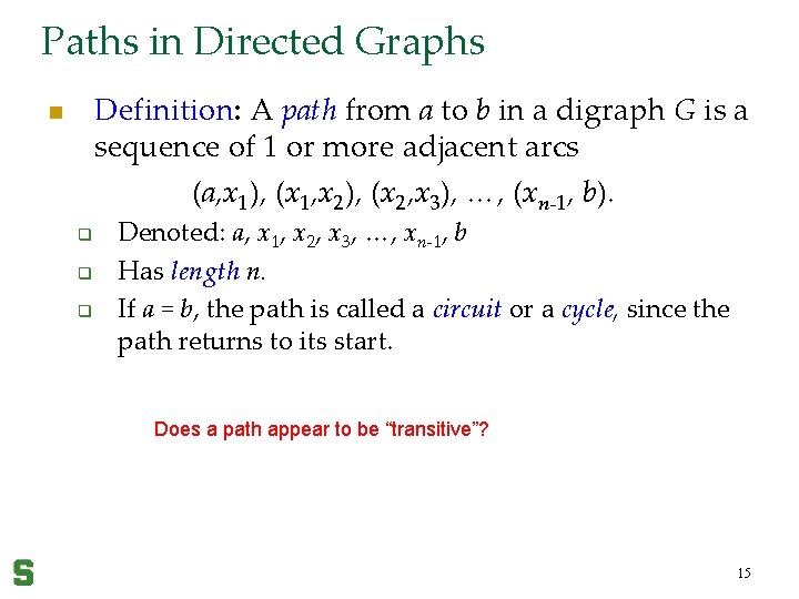
Paths in Directed Graphs Definition: A path from a to b in a digraph G is a sequence of 1 or more adjacent arcs (a, x 1), (x 1, x 2), (x 2, x 3), …, (xn-1, b). n q q q Denoted: a, x 1, x 2, x 3, …, xn-1, b Has length n. If a = b, the path is called a circuit or a cycle, since the path returns to its start. Does a path appear to be “transitive”? 15

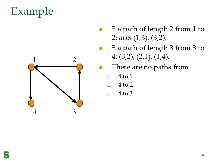
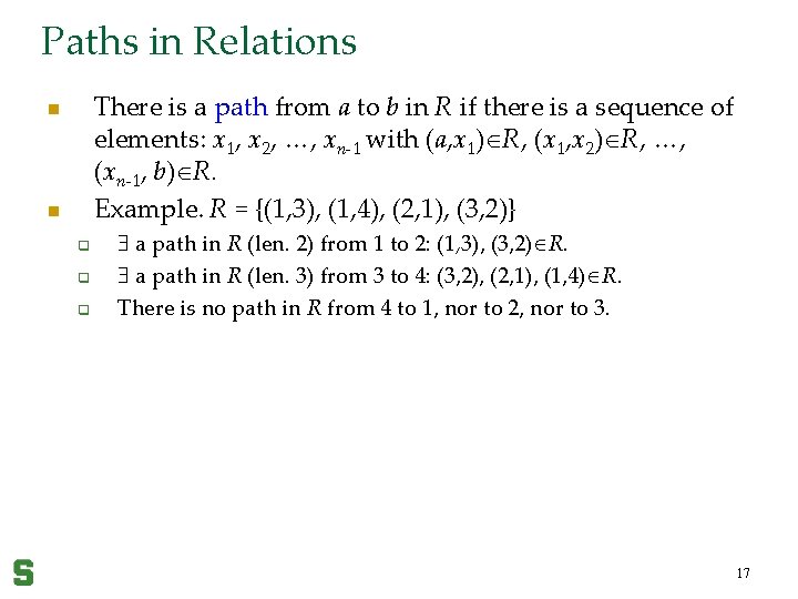
Example a path of length 2 from 1 to 2: arcs (1, 3), (3, 2). a path of length 3 from 3 to 4: (3, 2), (2, 1), (1, 4). There are no paths from n n 1 2 n q q q 4 4 to 1 4 to 2 4 to 3 3 16

Paths in Relations There is a path from a to b in R if there is a sequence of elements: x 1, x 2, …, xn-1 with (a, x 1) R, (x 1, x 2) R, …, (xn-1, b) R. Example. R = {(1, 3), (1, 4), (2, 1), (3, 2)} n n q q q a path in R (len. 2) from 1 to 2: (1, 3), (3, 2) R. a path in R (len. 3) from 3 to 4: (3, 2), (2, 1), (1, 4) R. There is no path in R from 4 to 1, nor to 2, nor to 3. 17

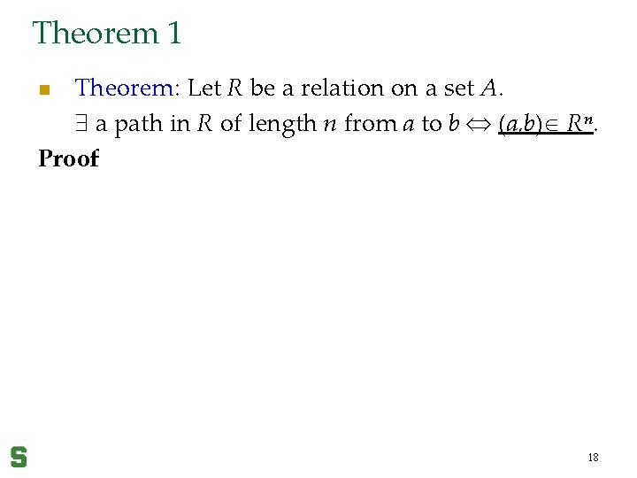
Theorem 1 Theorem: Let R be a relation on a set A. a path in R of length n from a to b (a, b) Rn. Proof n 18

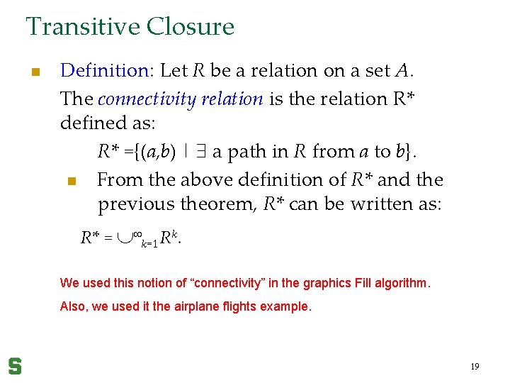
Transitive Closure n Definition: Let R be a relation on a set A. The connectivity relation is the relation R* defined as: R* ={(a, b) | a path in R from a to b}. n From the above definition of R* and the previous theorem, R* can be written as: R* = k=1 Rk. We used this notion of “connectivity” in the graphics Fill algorithm. Also, we used it the airplane flights example. 19

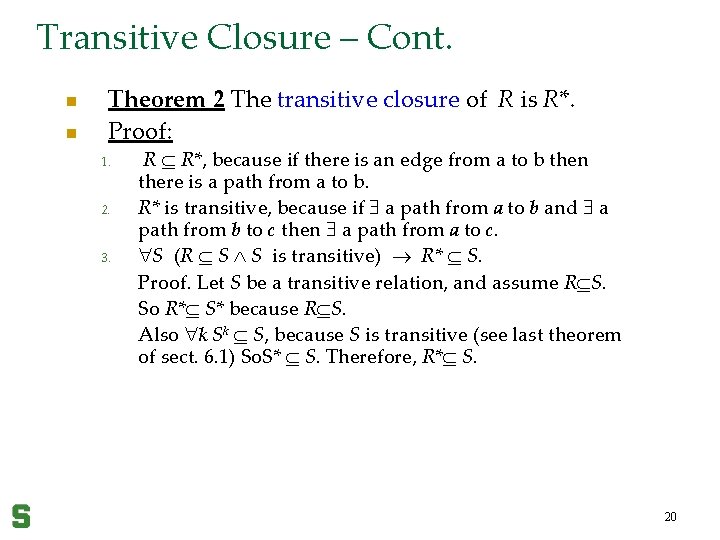
Transitive Closure – Cont. n n Theorem 2 The transitive closure of R is R*. Proof: 1. 2. 3. R R*, because if there is an edge from a to b then there is a path from a to b. R* is transitive, because if a path from a to b and a path from b to c then a path from a to c. S (R S S is transitive) R* S. Proof. Let S be a transitive relation, and assume R S. So R* S* because R S. Also k Sk S, because S is transitive (see last theorem of sect. 6. 1) So. S* S. Therefore, R* S. 20

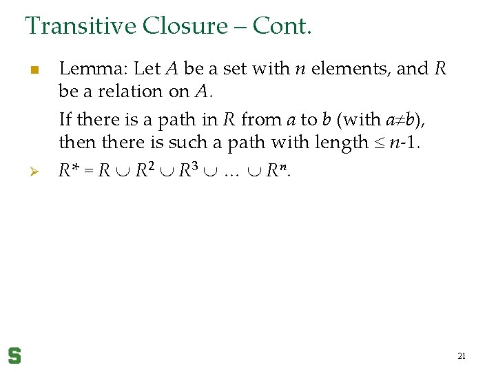
Transitive Closure – Cont. n Ø Lemma: Let A be a set with n elements, and R be a relation on A. If there is a path in R from a to b (with a b), then there is such a path with length n-1. R* = R R 2 R 3 … Rn. 21

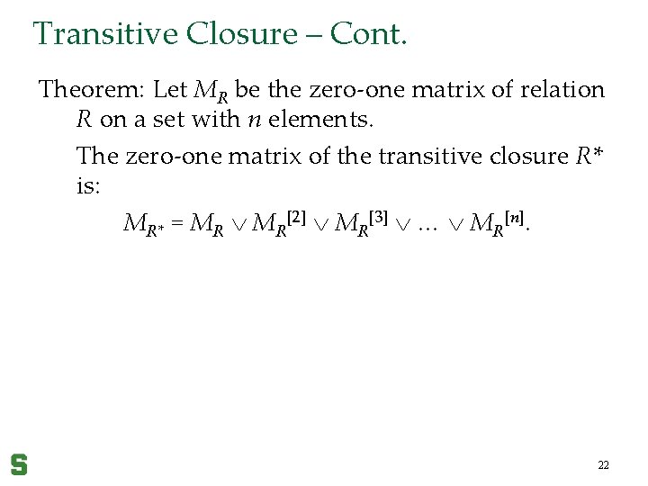
Transitive Closure – Cont. Theorem: Let MR be the zero-one matrix of relation R on a set with n elements. The zero-one matrix of the transitive closure R* is: MR* = MR MR[2] MR[3] … MR[n]. 22

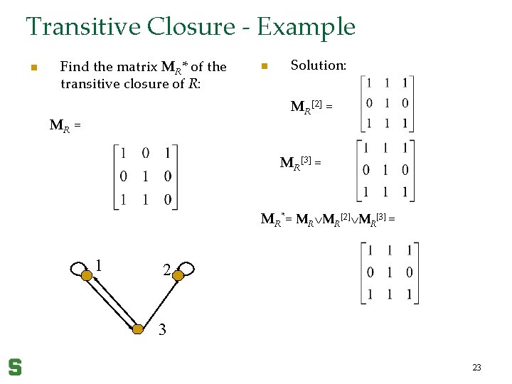
Transitive Closure - Example n Find the matrix MR* of the transitive closure of R: n Solution: MR[2] = MR[3] = MR*= MR MR[2] MR[3] = 1 2 3 23

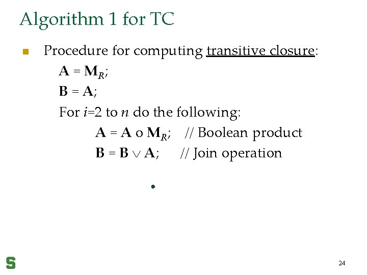
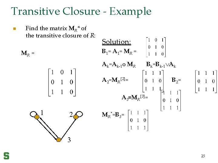
Algorithm 1 for TC n Procedure for computing transitive closure: A = MR; B = A; For i=2 to n do the following: A = A o MR; // Boolean product B = B A; // Join operation 24

Transitive Closure - Example n Find the matrix MR* of the transitive closure of R: Solution: B 1= A 1= MR = Ak=Ak-1 o MR Bk=Bk-1 Ak A 2=MR[2]= B 2 = A 3=MR[3]= 1 2 MR*=B 3= 3 25

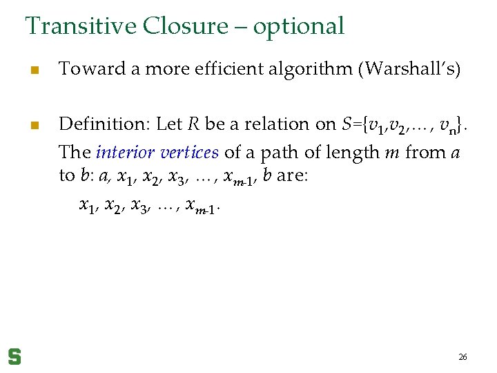
Transitive Closure – optional n n Toward a more efficient algorithm (Warshall’s) Definition: Let R be a relation on S={v 1, v 2, …, vn}. The interior vertices of a path of length m from a to b: a, x 1, x 2, x 3, …, xm-1, b are: x 1, x 2, x 3, …, xm-1. 26

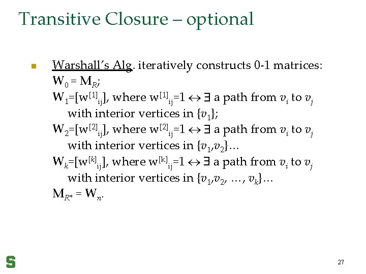
Transitive Closure – optional n Warshall’s Alg. iteratively constructs 0 -1 matrices: W 0 = MR; W 1=[w[1]ij], where w[1]ij=1 a path from vi to vj with interior vertices in {v 1}; W 2=[w[2]ij], where w[2]ij=1 a path from vi to vj with interior vertices in {v 1, v 2}… Wk=[w[k]ij], where w[k]ij=1 a path from vi to vj with interior vertices in {v 1, v 2, …, vk}… MR* = Wn. 27

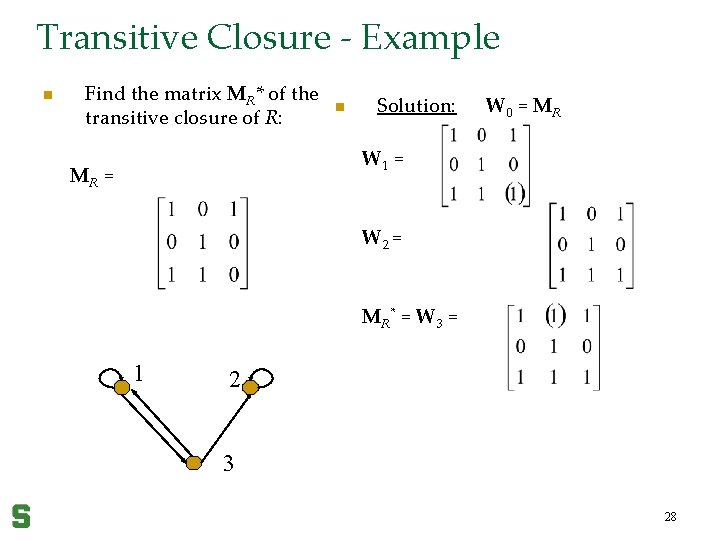
Transitive Closure - Example n Find the matrix MR* of the transitive closure of R: n Solution: W 0 = MR W 1 = MR = W 2 = MR* = W 3 = 1 2 3 28

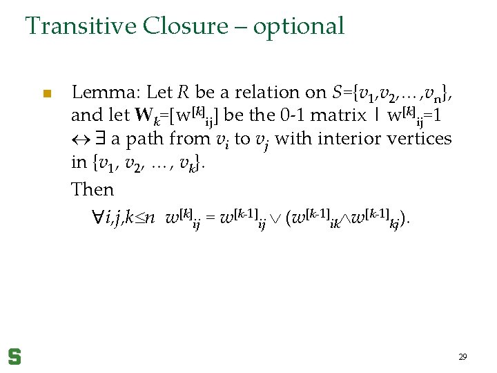
Transitive Closure – optional n Lemma: Let R be a relation on S={v 1, v 2, …, vn}, and let Wk=[w[k]ij] be the 0 -1 matrix | w[k]ij=1 a path from vi to vj with interior vertices in {v 1, v 2, …, vk}. Then i, j, k n w[k]ij = w[k-1]ij (w[k-1]ik w[k-1]kj). 29

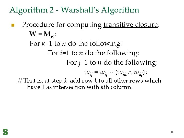
Algorithm 2 - Warshall’s Algorithm n Procedure for computing transitive closure: W = MR; For k=1 to n do the following: For i=1 to n do the following: For j=1 to n do the following: wij = wij (wik wkj); // That is, at step k: add row k to all other rows which have 1 as intersection with kth column. 30

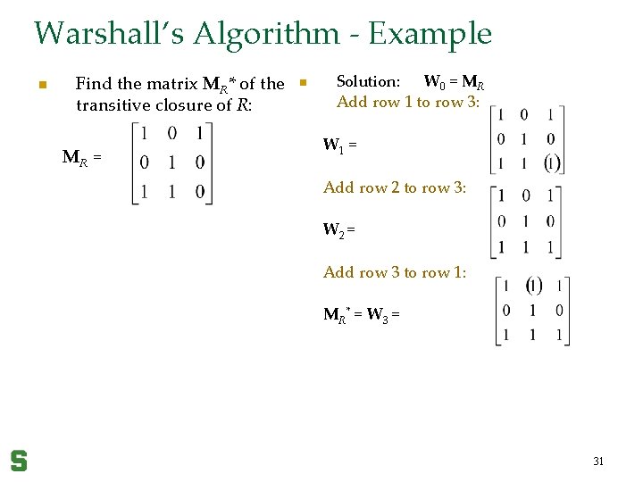
Warshall’s Algorithm - Example n Find the matrix MR* of the transitive closure of R: MR = n Solution: W 0 = MR Add row 1 to row 3: W 1 = Add row 2 to row 3: W 2 = Add row 3 to row 1: MR* = W 3 = 31

Conclusions: transitive closure Computing the transitive closure of a digraph is an important problem in many computer science applications: n q q q Evaluation of recursive database queries. Analysis of reachability (connectivity) of transition graphs in communication networks. Construction of parsing automata in compilers. 32

Equivalence relations These are reflexive, symmetric, and transitive. They partition the set of all elements into equivalence classes.

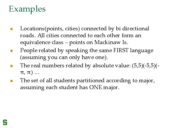
Examples n n Locations(points, cities) connected by bi directional roads. All cities connected to each other form an equivalence class – points on Mackinaw Is. People related by speaking the same FIRST language (assuming you can only have one). The real numbers related by absolute value: (5, 5)(-5, 5)(π, π) … The set of all students partitioned according to major, assuming each student has ONE major.

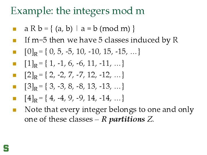
Example: the integers mod m n n n n a R b = { (a, b) | a ≡ b (mod m) } If m=5 then we have 5 classes induced by R [0]R = { 0, 5, -5, 10, -10, 15, -15, …} [1]R = { 1, -1, 6, -6, 11, -11, …} [2]R = { 2, -2, 7, -7, 12, -12, …} [3]R = { 3, -3, 8, -8, 13, -13, …} [4]R = { 4, -4, 9, -9, 14, -14, …} Note that every integer belongs to one and only one of these classes – R partitions Z.

Example: pixel adjacency partitions a binary image into “blobs” or “objects” 15 subsets of pixels. Within each subset, pixels are connected by a path through neighbors. Pixels in each subset are not connected to pixels in any other subset. (Connecting paths are not allowed to go through background pixels. )

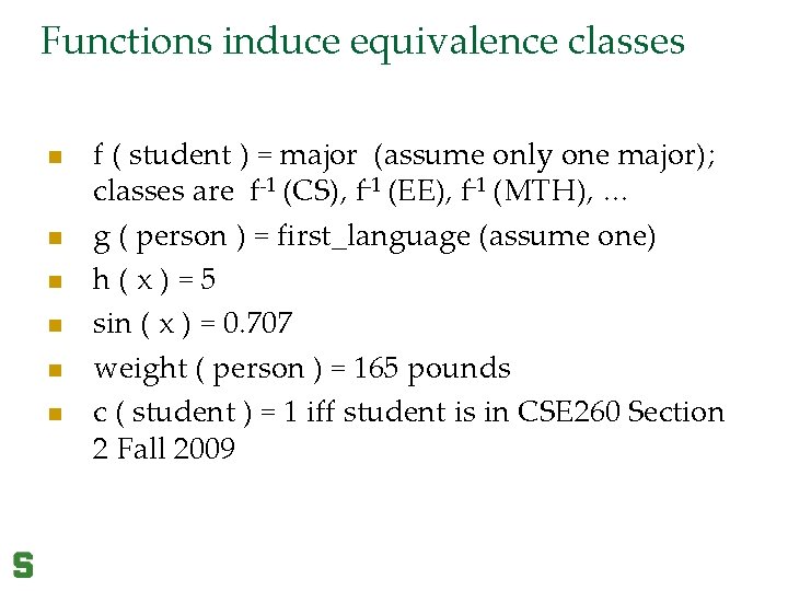
Functions induce equivalence classes n n n f ( student ) = major (assume only one major); classes are f-1 (CS), f-1 (EE), f-1 (MTH), … g ( person ) = first_language (assume one) h(x)=5 sin ( x ) = 0. 707 weight ( person ) = 165 pounds c ( student ) = 1 iff student is in CSE 260 Section 2 Fall 2009