Clocked Synchronous Statemachine Analysis Given the circuit diagram

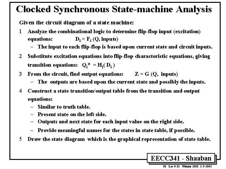
Clocked Synchronous State-machine Analysis Given the circuit diagram of a state machine: 1 Analyze the combinational logic to determine flip-flop input (excitation) equations: Di = Fi (Q, inputs) – The input to each flip-flop is based upon current state and circuit inputs. 2 Substitute excitation equations into flip-flop characteristic equations, giving transition equations: Qi* = Hi( Di ) 3 From the circuit, find output equations: Z = G (Q, inputs) – The outputs are based upon the current state and possibly the inputs. 4 Construct a state transition/output table from the transition and output equations: – Similar to truth table. – Present state on the left side. – Outputs and next state for each input value on the right side. – Provide meaningful names for the states in state table, if possible. 5 Draw the state diagram which is the graphical representation of state table. EECC 341 - Shaaban #1 Lec # 15 Winter 2001 2 -5 -2002

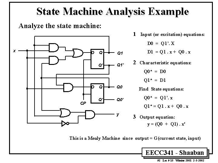
State Machine Analysis Example Analyze the state machine: 1 Input (or excitation) equations: D 0 = Q 1’. X x D Q Q 1 Q' Q 1' D 1 = Q 1. x + Q 0. x 2 Characteristic equations: Q 0* = D 0 Q 1* = D 1 D CP Q Q 0 Q' Q 0' Find State equations: Q 0* = Q 1’. x Q 1* = Q 1. x + Q 0. x y 3 Output equation: y = (Q 0 + Q 1). x' This is a Mealy Machine since output = G(current state, input) EECC 341 - Shaaban #2 Lec # 15 Winter 2001 2 -5 -2002

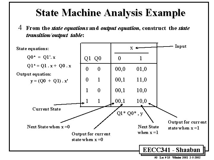
State Machine Analysis Example 4 From the state equations and output equation, construct the state transition/output table: Q 0* = Q 1’. x Q 1* = Q 1. x + Q 0. x Output equation: y = (Q 0 + Q 1). x' Input x State equations: Q 1 Q 0 0 1 0 0 00, 0 01, 0 0 1 00, 1 11, 0 1 0 00, 1 10, 0 1 1 00, 1 10, 0 Current State Q 1* Q 0* , y Next State when x =0 Output for current state when x =0 Next State when x =1 Output for current state when x =1 EECC 341 - Shaaban #3 Lec # 15 Winter 2001 2 -5 -2002

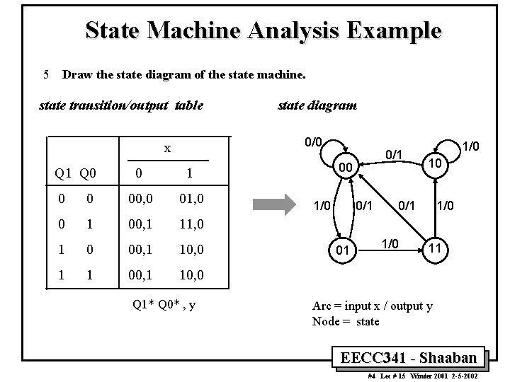
State Machine Analysis Example 5 Draw the state diagram of the state machine. state transition/output table 0/0 x Q 1 Q 0 state diagram 0 1 0 0 00, 0 01, 0 0 1 00, 1 11, 0 1 0 00, 1 10, 0 1 1 00, 1 10, 0 Q 1* Q 0* , y 0/1 00 1/0 0/1 01 1/0 10 0/1 1/0 11 Arc = input x / output y Node = state EECC 341 - Shaaban #4 Lec # 15 Winter 2001 2 -5 -2002

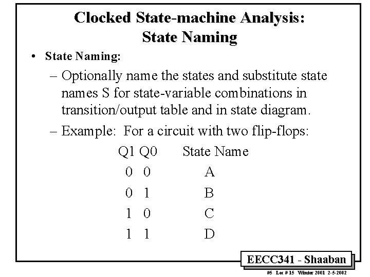
Clocked State-machine Analysis: State Naming • State Naming: – Optionally name the states and substitute state names S for state-variable combinations in transition/output table and in state diagram. – Example: For a circuit with two flip-flops: Q 1 Q 0 State Name 0 0 A 0 1 B 1 0 C 1 1 D EECC 341 - Shaaban #5 Lec # 15 Winter 2001 2 -5 -2002

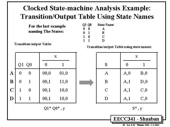
Clocked State-machine Analysis Example: Transition/Output Table Using State Names For the last example naming The States: Transition/output Table: Q 1 Q 0 0 1 1 State Name A B C D Transition/output Table using state names: x Q 1 Q 0 x 0 1 S 0 1 A 0 0 00, 0 01, 0 A A, 0 B 0 1 00, 1 11, 0 B A, 1 D, 0 C 1 0 00, 1 10, 0 C A, 1 C, 0 D 1 1 00, 1 10, 0 D A, 1 C, 0 Q 1* Q 0* , y S* , y EECC 341 - Shaaban #6 Lec # 15 Winter 2001 2 -5 -2002

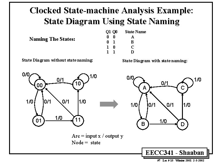
Clocked State-machine Analysis Example: State Diagram Using State Naming Q 1 Q 0 0 1 1 Naming The States: State Diagram without state naming: 0/0 0/1 00 1/0 0/1 01 0/1 1/0 State Name A B C D State Diagram with state naming: 1/0 10 1/0 11 0/0 0/1 A 1/0 0/1 B 0/1 1/0 C 1/0 D Arc = input x / output y Node = state EECC 341 - Shaaban #7 Lec # 15 Winter 2001 2 -5 -2002

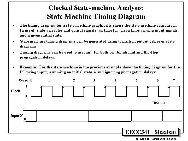
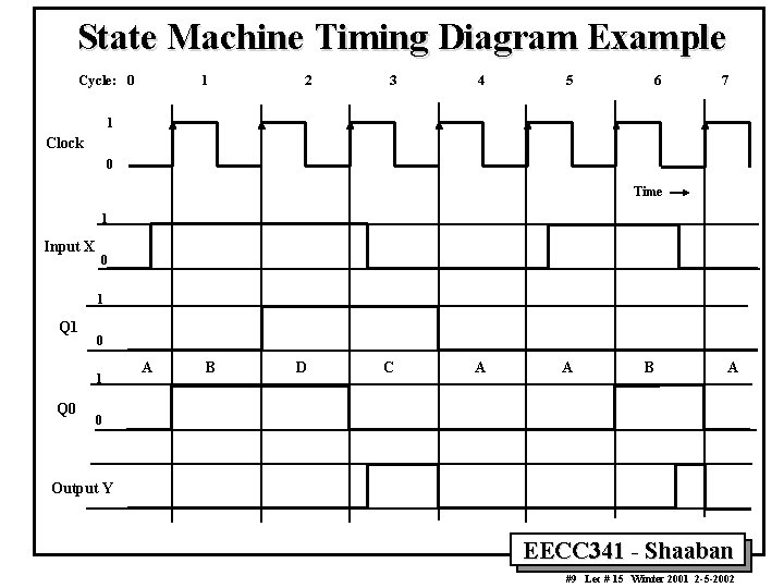
Clocked State-machine Analysis: State Machine Timing Diagram • • The timing diagram for a state machine graphically shows the state machine response in terms of state variables and output signals vs. time for given time-varying input signals and a given initial state. State machine timing diagrams can be generated using transition/output tables or state diagrams. Timing diagrams can be used to account for both combinational and flip-flop propagation delays. Example: For the state machine in the previous example show the timing diagram for the following input, assuming an initial state A and ignoring propagation delays: Cycle: 0 1 2 3 4 5 6 7 1 Clock 0 Time 1 Input X 0 EECC 341 - Shaaban #8 Lec # 15 Winter 2001 2 -5 -2002

State Machine Timing Diagram Example Cycle: 0 1 2 3 4 5 6 7 1 Clock 0 Time 1 Input X 0 1 Q 1 0 1 Q 0 A B D C A A B A 0 Output Y EECC 341 - Shaaban #9 Lec # 15 Winter 2001 2 -5 -2002

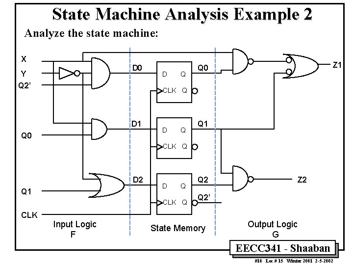
State Machine Analysis Example 2 Analyze the state machine: X D 0 Y Q 2’ D Q Z 1 Q 0 CLK Q D 1 Q 0 D Q Q 1 CLK Q D 2 Q 1 D Q CLK Input Logic F Q 2 Z 2 Q 2’ State Memory Output Logic G EECC 341 - Shaaban #10 Lec # 15 Winter 2001 2 -5 -2002

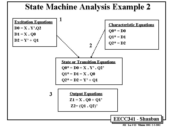
State Machine Analysis Example 2 Excitation Equations D 0 = X. Y’. Q 2 D 1 = X. Q 0 D 2 = Y’ + Q 1 1 2 Characteristic Equations Q 0* = D 0 Q 1* = D 1 Q 2* = D 2 State or Transition Equations Q 0* = D 0 = X. Y’. Q 2’ Q 1* = D 1 = X. Q 0 Q 2* = D 2 = Y’ + Q 1 3 Output Equations Z 1 = X. Q 0 + Q 1’ Z 2= (Q 1. Q 2)’ EECC 341 - Shaaban #11 Lec # 15 Winter 2001 2 -5 -2002

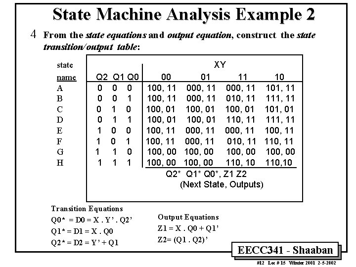
State Machine Analysis Example 2 4 From the state equations and output equation, construct the state transition/output table: state name A B C D E F G H XY Q 2 0 0 1 1 Q 1 Q 0 0 1 1 0 0 0 1 1 Transition Equations Q 0* = D 0 = X. Y’. Q 2’ Q 1* = D 1 = X. Q 0 Q 2* = D 2 = Y’ + Q 1 00 01 11 10 100, 11 000, 11 101, 11 100, 11 010, 11 111, 11 100, 01 101, 01 100, 01 110, 11 111, 11 100, 11 000, 11 100, 11 010, 11 100, 00 100, 00 110, 10 Q 2* Q 1* Q 0*, Z 1 Z 2 (Next State, Outputs) Output Equations Z 1 = X. Q 0 + Q 1’ Z 2= (Q 1. Q 2)’ EECC 341 - Shaaban #12 Lec # 15 Winter 2001 2 -5 -2002

State-machine Analysis Example 2: Transition/Output Table Using State Names XY S A B C D E F G H 00 E, 11 E, 01 E, 11 E, 00 01 11 A, 11 C, 11 E, 01 G, 11 A, 11 C, 11 E, 00 G, 10 S*, Z 1 Z 2 10 F, 11 H, 11 F, 01 H, 11 E, 11 G, 11 E, 00 G, 10 EECC 341 - Shaaban #13 Lec # 15 Winter 2001 2 -5 -2002

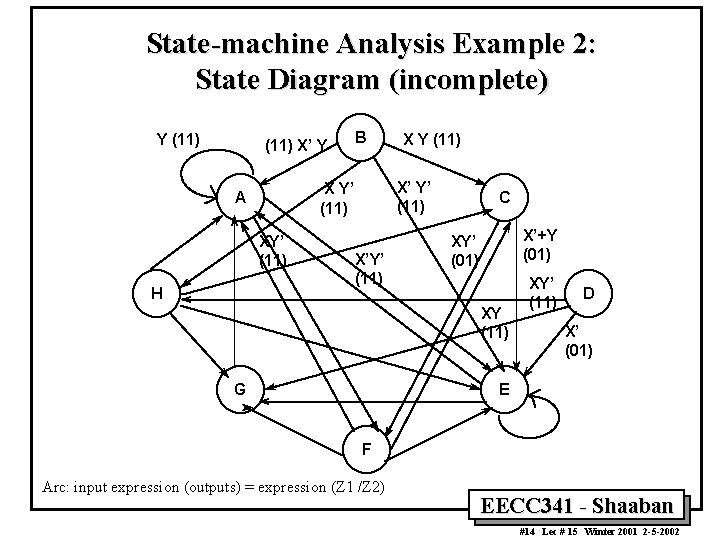
State-machine Analysis Example 2: State Diagram (incomplete) Y (11) X’ Y XY’ (11) X Y (11) X’ Y’ (11) X Y’ (11) A H B X’Y’ (11) C X’+Y (01) XY’ (01) XY (11) G XY’ (11) D X’ (01) E F Arc: input expression (outputs) = expression (Z 1 /Z 2) EECC 341 - Shaaban #14 Lec # 15 Winter 2001 2 -5 -2002

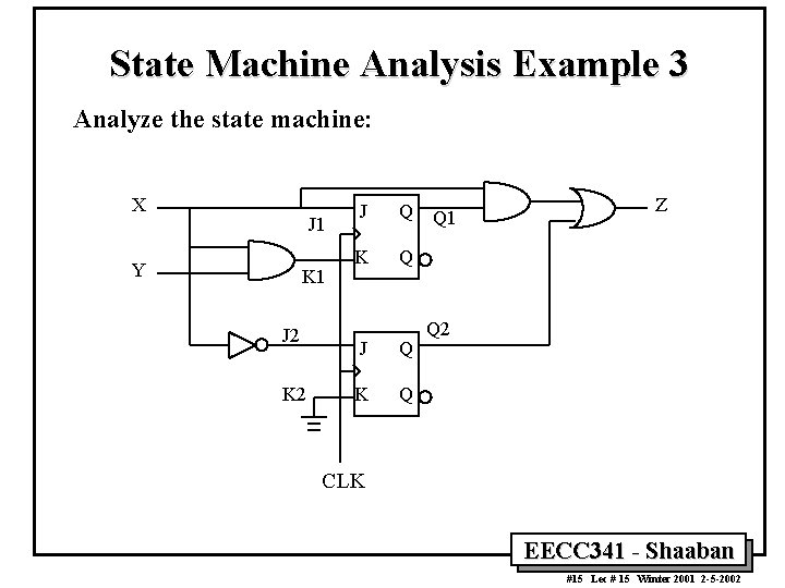
State Machine Analysis Example 3 Analyze the state machine: X J 1 Y K 1 J 2 K 2 J Q K Q Q 1 Z Q 2 CLK EECC 341 - Shaaban #15 Lec # 15 Winter 2001 2 -5 -2002

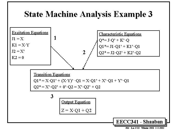
State Machine Analysis Example 3 Excitation Equations J 1 = X K 1 = X·Y J 2 = X’ K 2 = 0 1 2 Characteristic Equations Q*= J·Q’ + K’·Q Q 1*= J 1·Q 1’ + K 1’·Q 1 Q 2* = J 2·Q 2’ + K 2’·Q 2 Transition Equations Q 1* = X·Q 1’ + (X·Y)’ ·Q 1 = X·Q 1’ + X’·Q 1 + Y’·Q 1 Q 2* = X’·Q 2’ + 0’·Q 2 = X’·Q 2’ + Q 2 3 Output Equation Z = X·Q 1 + Q 2 EECC 341 - Shaaban #16 Lec # 15 Winter 2001 2 -5 -2002

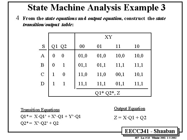
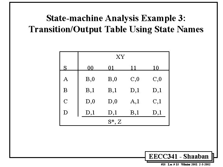
State Machine Analysis Example 3 4 From the state equations and output equation, construct the state transition/output table: XY S Q 1 Q 2 00 01 11 10 A 0 0 01, 0 10, 0 B 0 1 01, 1 11, 1 C 1 0 11, 0 00, 1 10, 1 D 1 1 11, 1 01, 1 11, 1 Q 1* Q 2*, Z Transition Equations Q 1* = X·Q 1’ + X’·Q 1 + Y’·Q 1 Q 2* = X’·Q 2’ + Q 2 Output Equation Z = X·Q 1 + Q 2 EECC 341 - Shaaban #17 Lec # 15 Winter 2001 2 -5 -2002

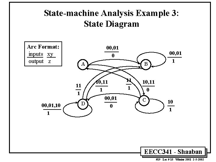
State-machine Analysis Example 3: Transition/Output Table Using State Names XY S 00 01 11 10 A B, 0 C, 0 B B, 1 D, 1 C D, 0 A, 1 C, 1 D D, 1 B, 1 D, 1 S*, Z EECC 341 - Shaaban #18 Lec # 15 Winter 2001 2 -5 -2002

State-machine Analysis Example 3: State Diagram Arc Format: inputs xy output z 00, 01 0 A 10, 11 1 00, 01, 10 1 B D 00, 01 0 11 1 00, 01 1 10, 11 0 C 10 1 EECC 341 - Shaaban #19 Lec # 15 Winter 2001 2 -5 -2002