Climate models Ren D Garreaud Departement of Geophysics

Climate models René D. Garreaud Departement of Geophysics Universidad de Chile www. dgf. uchile. cl/rene

Modelación Numérica de la Atmósfera • • • ¿Por que empleamos modelos climáticos? ¿En que consiste un modelo climático? ¿Qué son variables y parámetros? ¿Qué son los GCM, AOGCM y RCM? Aplicaciones y limitaciones

¿Porque empleamos modelos climáticos? • Suplemento de observaciones climáticas (interpolación física). Aunque son una representación incompleta del mundo real, un buen modelo captura gran parte de la dinámica del sistema climático terrestre. • Experimentos de gran escala (cambio en forzantes) y análisis de sensibilidad. • Generación de escenarios climáticos pasados y futuros. Los números que entrega un modelo pueden no ser “exactos” pero dan un rango plausible de cambio climático pasados o futuros. • Dynamical downscaling (escalamiento hacia abajo basado) de climas pasados y futuros. • Método alternativo (modelos conceptuales cualitativos) aguanta cualquier cosa…

¿Porque me gustan tanto las modelos? • Aunque son una representación incompleta del mundo real, un buen modelo captura gran parte de la dinámica del sistema climático terrestre. • Método alternativo (modelos conceptuales cualitativos) aguanta cualquier cosa… • Los números que entrega un modelo pueden no ser “exactos” pero dan un rango plausible de cambio climático pasados o futuros.

Sistema Terrestre Todos juntos y al mismo tiempo Espacio Exterior Criosfera Atmósfera Biosfera Hidrosfera Litosfera

Sistema Terrestre Subsistema Tiempo de ajuste a cambio climático de escala global Océano superficial Meses - Años Océano Profundo Años - Décadas Campos de Hielo Años - Décadas Biosfera continental Años - Décadas Litosfera > Miles de años

Mayor largo de simulacion requiere incorporar mas subsistemas terrestres a la simulacion (variables vs parámetros) hasta llegar a modelos del sistema terrestre completo (atmos-ocean-crio-bio-lito) d. T = dias-años d. T = años - décadas d. T = siglos y + Atmosfera Oceano Superficial Oceano Profundo Sistema Modelado Prescrito

Complexity Global Models (GCM) Type SST Sea Ice Land Ice Biosphere Land use AGCM P P P AOGCM C C P P P CGCM C C C P P ESM C C C 1980 - 1990 - 2005 - A: Atmospheric Only; C: Coupled; O: Ocean; ESM: Earth-system models External parameters: GHG, O 3, aerosols concentration; solar forcing

Global Circulation Models (GCM)

My first toy model A system of coupled, non-linear algebraic equations X(t) = A·X(t-1) ·Y(t) + B·Z(t-1) + x Y(t)= C·X(t-1)·Y (t-1) + B·Z (t)+ y Z(t)= D·Z(t-1)·Y (t) + E·X(t-1) + z x = y = z = 0 X, Y, Z: Time-dependent variables Pressure, winds, temperature, moisture, …. A, B, C, D: External parameter Orbital parameters, CO 2 Concentration, SST (AGCM), Land cover x y z Randoms error Set to zero Deterministic model

My first toy model X(t) = A·X(t-1) ·Y(t) + B·Z(t-1) + x Y(t)= C·X(t-1)·Y (t-1) + B·Z (t)+ y Z(t)= D·Z(t-1)·Y (t) + E·X(t-1) + z x = y = z = 0 To run the model, we need: • Initial conditions: X 0, Y 0, Z 0 • The values of the External Parameters … they can vary on time • A numerical algorithm to solve the equations • A computer big enough

Mod Weather forecast Model predicts daily values Obs Climate Prediction Model does NOT predict daily values but still gives reasonable climate state (mean, variance, spectra, etc…)

The Lorenz’s (butterfly) chaos effect X 0 = -0. 501 X 0 = -0. 502 A slight difference in the initial conditions Non-linear equations Large differences later on

Nevertheless, simulations after two-weeks are still “correct” in a climatic perspective and highly dependent upon external parameters models can be used to see how the climate changes as external parameters vary. A=2 A=1 Two runs of the model, everything equal but parameter A. Note the “Climate Change” related to change in A The climate change signal is more robust when using the mean of an ensemble (several runs with slightly different IC). In doing this, however, extreme events are lost

Examples of External Parameters that can be modified: 1. The relatively long memory of tropical SST can be used to obtain an idea of the SST field in the next few months (e. g. , El Niño conditions). Using this predicted SST field to force an AGCM, allows us climate outlooks one season ahead. 2. Changes in solar forcing (due to changes in sun-earth geometry) are very well known for the past and future (For instance, NH seasonality was more intense in the Holocene than today). Modification of this parameter allow us paleo-climate reconstructions (still need to prescribe other parameters in a consistent way: Ice cover, SST, etc. …hard!) 3. Changes in greenhouse gases concentration in the next decades gases give us some future climate scenarios.

Atmospheric circulation is governed by fluid dynamics equation + ideal gas thermodynamics Momentum eqn. Energy eqn. Mass eqn. Idea gas law Water substance eqns.

¿¿¿Where is precipitation? ? ? d ou m W ar Ice crystal Rain droplets Snow Graupel/Hail s Cloud droplets d ou cl cl ld Co Water Vapor

Previous system is highly non-linear, with no simple analytic solution ? !. . We solve the system using numerical methods applied upon a three-dimensional grid

Once selected the domain and grid, the numerical integration uses finite differences in time and space Numerial method (stable & efficient) Sub-grid processes must be parameterized, that is specified in term of large-scale variables

Global Models (GCM) z lat lon lat ~ lon ~ 1 - 3 z ~ 1 km t ~ minutes-hours Top of atmosphere: 15 -50 km

Ejemplo 1: Cambio climático antropogénico (siglo XXI) Parámetros variables: Concentración de gases con efecto invernadero. Parámetros fijos: Geografía, geometría tierra sol. Componentes variables: Circulación atmosférica y oceánica, biosfera simplificada

EJEMPLO 1: Clima del Siglo XXI Escenarios Desarrollo Economico-Social GCMs

EJEMPLO 1 © IPCC 2007: WG 1 -AR 4 (2007)

EJEMPLO 1 © IPCC 2007: WG 1 -AR 4 (2007)

Ejemplo 2: Clima del Cretáceo Parámetros “alterados”: Concentración de gases con efecto invernadero, geografía, geometría tierra sol. Componentes variables: Circulación atmosférica y oceánica, biosfera simplificada

Ruddiman: Earth’s Climate, Chapter 4 Early Cretaceous world

Modelos además presentan problemas en climas pasados Termostato tropical? Múltiples equilibrios? GCMs (cambios CO 2 + geografía) Ruddiman: Earth’s Climate, Chapter 4

La aparente existencia de un termostato tropical y su no representación en GCMs es un problema… Sin embargo una buena culebra ayuda Head et al. Nature 2009

Head et al. Nature 2009

Head et al. Nature 2009

Reconstrucción incluyendo Titanoboa otorga más credibilidad a GCMs Reconstrucción c/culebra GCMs (cambios CO 2 + geografía) Ruddiman: Earth’s Climate, Chapter 4

Ejemplo 3: Aridificación del desierto de Atacama En este caso haremos un experimento de sensibilidad y no una simulación paleo-climática. No es necesario alcanzar equilibrio. Parámetros “alterados”: geografía (Andes) y temperatura superficial del oceano. Parametros fijos: Concentración GEI, geometría tierrasol, TSM, geografía. Componentes variables: Circulación atmosférica.

High Andes & dry Atacama Iquique 6 mm/década Calama 12 mm/decada Condiciones actuales hiper-áridas a lo largo del desierto costero. Sin embargo, abundante evidencia geológica de un pasado remoto (Ma) menos extremo en cuanto a déficit de precipitación (e. g. , formación de yacimientos de Cu)

High Andes & dry Atacama Posicionamiento de Sud América en rango actual de latitudes (80 -100 Ma)

Conceptually, both Andean uplift (enhanced bloking of moist air) and SEP cooling (less evaporation from ocean) may increase dryness of the Atacama desert…it would be nice to use a “simple” climate model to study these two conditions. We use PLASIM, an Earth System Model of Intermediate Complexity from Hamburg University: • Atmospheric component: PUMA • Simple slab model for SST and Sea Ice • SIMBA for biosphere We performed 50 year long simulations altering one Boundary condition at a time

Model Validation

PLASIM Topography Experiments 0. 3*Topo minus Control (DJF) 900 h. Pa winds and Precip % Precip ( P/Pc)

PLASIM “Humboldt” Experiments u. SST: SST( ) only w. SEP: warmer Southeast Pacific

PLASIM “Humboldt” Experiments u. SST minus Control (DJF) 900 h. Pa winds and Precip % Precip ( P/Pc)

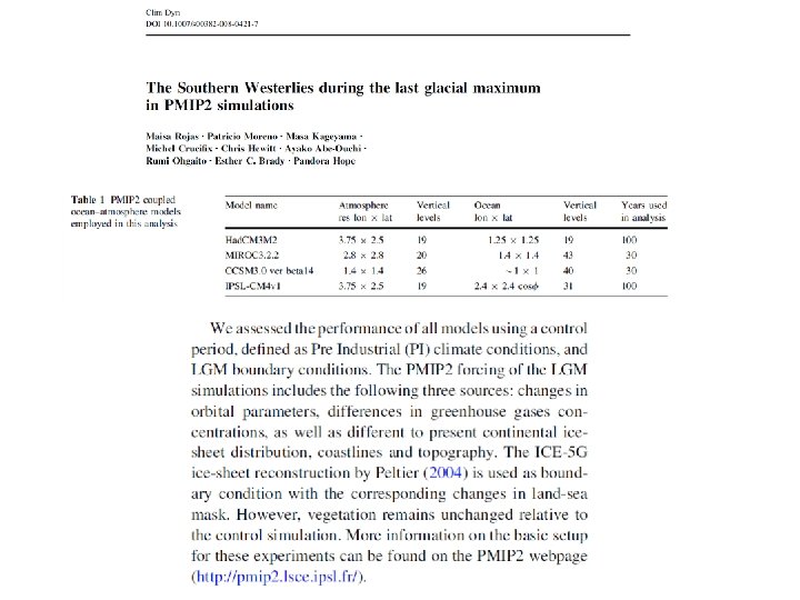
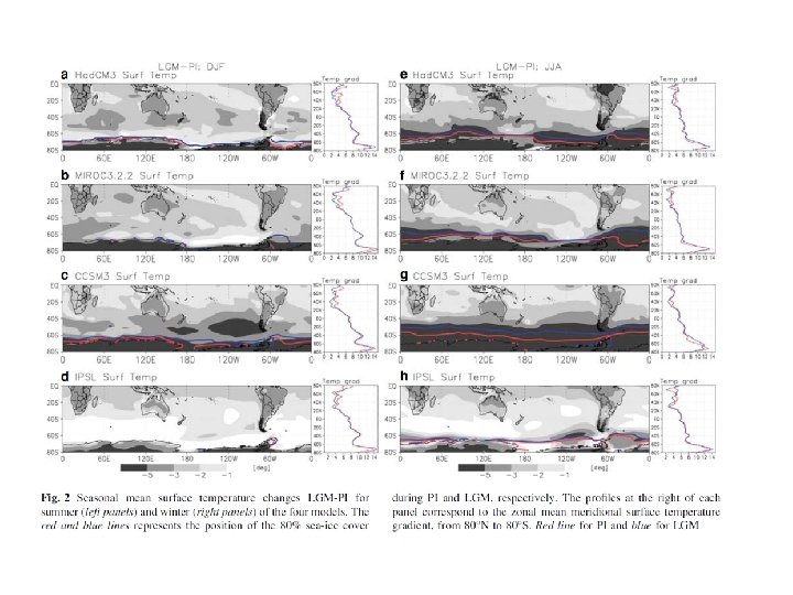
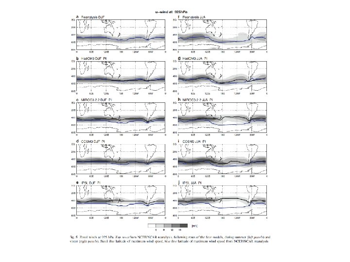
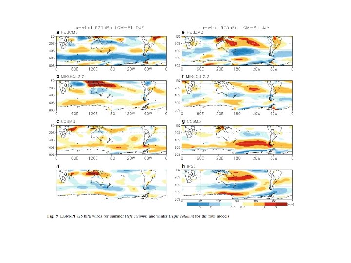
Ejemplo 4: Clima durante el LGM

Regional Models (LAM, MM) Lx z Ly y Lz x x ~ y ~ 1 -50 km z ~ 50 -200 m t ~ seconds Lx ~ L y ~ 100 -5000 km Lz ~ 15 km

Regional Models (LAM, MM) Regional models gives us a lot more detail (including topographic effects) but they need to be “feeded” at their lateral boundaries by results from a GCM. Main problem: Garbage in – Garbage out

Proyecto CONAMA – DGF/UCH http: //www. dgf. uchile. cl/PRECIS Model: • PRECIS – UK Single domain • Horiz. grid spacing. 25 km • 19 vertical levels • Lateral BC: Had. AM every 6 h • Sfc. BC: Had. ISST 1 + Linear trend Simulations • 1961 -1990 Baseline • 2071 -2100 SRES A 2 y B 2 • 30 years @ 3 min 4 months per simulation in fast PC

Surface Temperature Difference A 2 -BL 30°S 75°W -1° 0° 1° 2° 3° 4° 5° C 50°S

Precipitation Difference A 2 -BL -50 30°S 50°S 75°W 0 +50 mm/mes