CLIM 101 Weather Climate and Global Society What

CLIM 101: Weather, Climate and Global Society What is a climate model? If we cannot predict weather, how can we predict climate? Jagadish Shukla Lecture 11: Oct 6, 2009

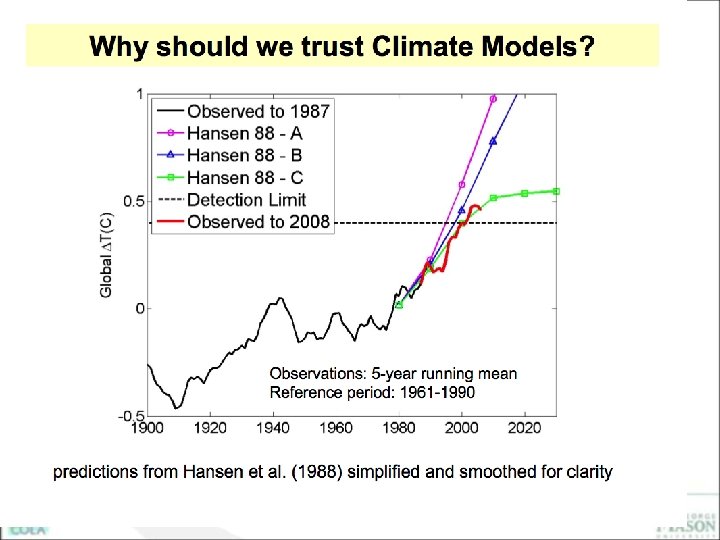
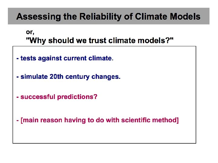
Reading for Week 6 Lecture 11 What is a climate model? • GW Chapter 5 • IPCC WG 1 Chapter 8, FAQ 8. 1 How Reliable Are the Models Used to Make Projections of Future Climate Change?

Intergovernmental Panel on Climate Change (IPCC) IPCC has been established by WMO and UNEP to assess scientific, technical and socio- economic information relevant for the understanding of climate change, its potential impacts and options for adaptation and mitigation. Working Group I: The Physical Science Basis Working Group II: Impacts, Adaptation and Vulnerability Working Group III: Mitigation of Climate Change • Largest number of U. S. scientists: nominated by the U. S. Govt. • Highest skepticism : “U. S. Govt. ”

What is a Model? • Quantitative and/or qualitative representation of natural processes (may be physical or mathematical) • Based on theory • Suitable for testing “What if…? ” hypotheses • Capable of making predictions

What is a Model? Input Data Model What input data might we consider for a typical climate model? Output Data What output data might we consider for a typical climate model? Tunable Parameters What are the tunable parameters of interest?

Climate System Modeling Atmospheric General Circulation Model Physical processes Dynamics Basic Equations

Ω CLIMATE DYNAMICS OF THE PLANET EARTH g S a (albedo) T 4 O 3 S, H 2 O , a, g, Ω CO 2 h*: mountains, oceans (SST) w*: forest, desert (soil wetness) stationary waves (Q, h*), monsoons hydrodynamic instabilities of shear flows; stratification & rotation; moist thermodynamics day-to-day weather fluctuations; wavelike motions: wavelength, period, amplitude W E A T H E R C L I M A T E.

Newton’s law Energy conservation Mass conservation (approximation) = p / ps

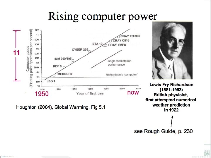
What is a Climate Model? • Equations of motions and laws of thermodynamics to predict rate of change of: T, P, V, q, etc. (A, O, L, CO 2, etc. ) • 10 Million Equations: 100, 000 Points × 100 Levels × 10 Variables • With Time Steps of: ~ 10 Minutes • Use Supercomputers

Discretization Atmosphere and ocean are continuous fluids … but computers can only represent discrete objects

ENIAC IBM 360 Columbia NASA John von Neumann Seymour Cray & Cray-1 Cray-2

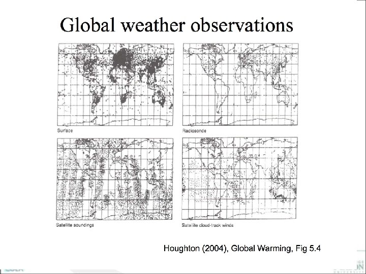
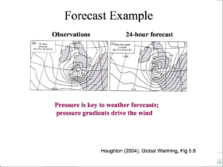
Weather Prediction Future pressure = current pressure + (rate of change of pressure) x t Future temperature = current temp. + (rate of change of temp. ) x t Current pressure & temperature: use global observations For rate of change: use mathematical equations For producing forecast: use supercomputers

Sea Level Pressure (mb) & Precipitation Rate (mm/12 Hr) 00 Z Tue 10 Nov 1998

Sea Level Pressure (mb) & Precipitation Rate (mm/12 Hr) 12 Z Tue 10 Nov 1998

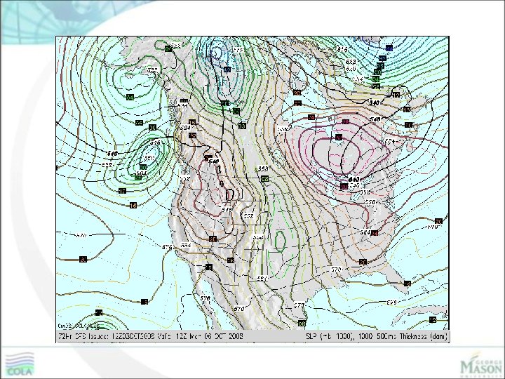
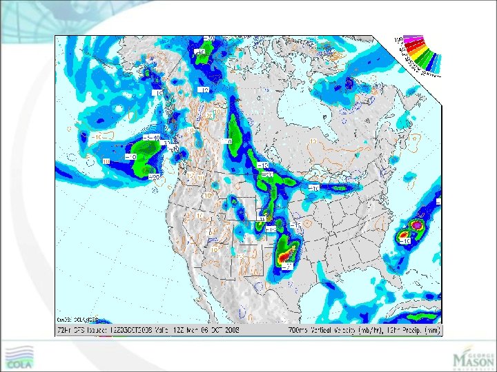
Sea Level Pressure (mb) & Precipitation Rate (mm/12 Hr) 00 Z Wed 11 Nov 1998

Numerical Weather Prediction 1. Determine (continuous) equations to be solved – – – 2. 3. 4. 5. Equation of state or Ideal Gas Law (Boyle’s Law relates P V, Charles’ Law relates V T, Gay-Lussac’s Law relates T P) Conservation of mass (dry air, water) Conservation of energy Conservation of angular momentum Result: set of coupled, nonlinear, partial differential equations Discretize the equations for numerical solution (typically requires computer) Measure current state of global atmosphere to obtain initial conditions Solve the initial value problem to produce a forecast Take into account uncertainty in measured atmospheric state by repeating step 4 over an ensemble of slightly different initial conditions

Science 23 October 1998, Volume 282, pp. 728 -731 Predictability in the Midst of Chaos: A Scientific Basis for Climate Forecasting J. Shukla Soil Wetness SST Anomalies (o. C)

El Nino/Southern Oscillation 1998 JFM SST [o. C] JFM SST Climatology [o. C] 1998 JFM SST Anomaly [o. C]

El Nino/Southern Oscillation

Rainfall Anomalies

Model Simulation of ENSO Effects 500 h. Pa Height Anomalies (ACC = 0. 98) Vintage 2000 AGCM

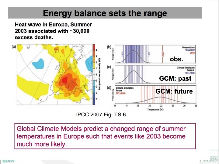
European Heat Wave 2003

JJA 2003 SST Anomaly

JJA obs OBS. SST-CLIM. SST exp. result significant at more than 90% sig. lev.

GEC is more acute than ever • Heat wave hits • Europe • 30, 000 people die • in Western Europe Temperature anomaly (wrt 1961 -90) °C • 2003 observations Had. CM 3 Medium-High (SRES A 2) 2003 2060 s 2040 s

Courtesy of P. Houser (GMU)

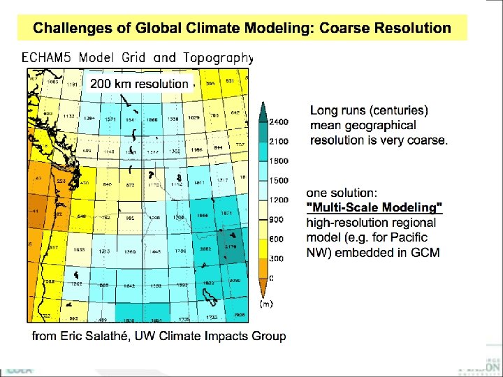
200 km

Computing Capability & Global Model Grid Size (km) Peak Rate: 10 TFLOPS 100 TFLOPS 1 PFLOPS 100 PFLOPS 1, 400 (2006) 12, 000 (2008) 80 -100, 000 (2009) 300 -800, 000 (2011) 6, 000? (20 xx? ) Global NWP 0: 5 -10 days/hr 18 - 29 8. 5 - 14 1. 8 - 2. 9 0. 85 - 1. 4 Seasonal 1: 50 -100 days/day 17 - 28 8. 0 - 13 1. 7 - 2. 8 0. 80 - 1. 3 Decadal 1: 5 -10 yrs/day 57 - 91 27 - 42 5. 7 - 9. 1 2. 7 - 4. 2 12 - 20 5. 7 - 9. 1 Cores (1 st year available) Climate Change 2: 120 - 200 20 -50 yrs/day Range: Assumed efficiency of 10 -40% 57 - 91 0 - Atmospheric General Circulation Model (AGCM; 100 levels) 1 - Coupled Ocean-Atmosphere-Land Model (CGCM; ~ 2 X AGCM computation with 100 -level OGCM) 2 - Earth System Model (ESM; ~ 2 X CGCM computation) 4. 0 - 6. 3 (~20 X 106 points) 3. 7 - 5. 9 (~20 X 106 points) 12 - 20 (~2 X 106 points) 27 - 42 (~0. 5 X 106 points) * Core counts above O(104) are unprecedented for weather or climate codes, so the last 3 columns require getting 3 orders of magnitude in scalable parallelization (scalar processors assumed; vector processors would have lower processor counts) Thanks to Jim Abeles (IBM)

• Geographic resolution characteristic of the generations of climate models used in the IPCC Assessment Reports: FAR (IPCC, 1990), SAR (IPCC, 1996), TAR (IPCC, 2001 a), and AR 4 (2007). • The figures above show successive generations of these global models increasingly resolved northern Europe. These illustrations are representative of the most detailed horizontal resolution used for short-term climate simulations. • The century-long simulations cited in IPCC Assessment Reports after the FAR were typically run with the previous generation’s resolution. Vertical resolution in both atmosphere and ocean models is not shown, but it has increased comparably with the horizontal resolution, beginning typically with a singlelayer slab ocean and ten atmospheric layers in the FAR and progressing to about thirty levels in both atmosphere and ocean.

Projection of Global Warming Mean of 15 Models Surface Air Temperature Difference (Sresa 1 b YR 71 -100) minus (20 c 3 m 1969 -98), Global Average = 2. 61 Center of Ocean-Land. Atmosphere studies

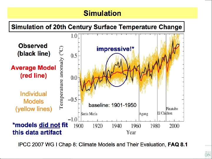
Increase in Surface Temperature Observations Predictions with Anthropogenic/Natural forcings Predictions with Natrual forcings 1. 0º C IPCC 2007

Climate Model Fidelity and Projections of Climate Change J. Shukla, T. Del. Sole, M. Fennessy, J. Kinter and D. Paolino Geophys. Research Letters, 33, doi 10. 1029/2005 GL 025579, 2006 Center of Ocean-Land. Atmosphere studies

Summary 1. Weather prediction depends on initial conditions (global observations). 2. Short-term climate (seasonal-decadal) depends on boundary conditions (SST, soil wetness, snow, sea ice, etc. ), which depends on ocean-atmosphere interactions. (natural forcings: sun, volcanoes, etc. ) 3. Long-term climate change depends on “exteranal” forcings (Human: greenhouse gases, land cover change, etc. )

THANK YOU! ANY QUESTIONS?