Cli MAF Earth System Model Evaluation Platform Evaluatingcomparing

Cli. MAF Earth System Model Evaluation Platform Evaluating/comparing a set of simulations/models on Ciclad: Demo / TP 1

Outline C-ESM-EP Demo / Practicals 1. Running the C-ESM-EP demo for all components 1. Atlas Explorer as an exploratory tool: 1. Modify the input datasets: 1. Add/modify datasets (CMIP 5 models or IGCM_OUT simulations) 2. Change the period and frequency 3. Setup your own Cli. MAF project 4. Control the reference 2. Using the Atlas Explorer parameter file 1. Overall parameters 2. Play with the dictionaries of the variables 3. Add new variables 4. Modify the plot parameters 2

1. Running The C-ESM-EP 3

4

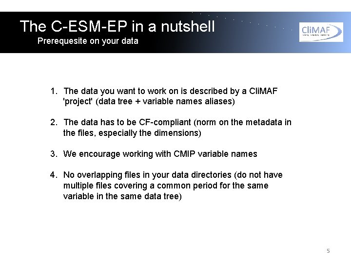
The C-ESM-EP in a nutshell Prerequesite on your data 1. The data you want to work on is described by a Cli. MAF 'project' (data tree + variable names aliases) 2. The data has to be CF-compliant (norm on the metadata in the files, especially the dimensions) 3. We encourage working with CMIP variable names 4. No overlapping files in your data directories (do not have multiple files covering a common period for the same variable in the same data tree) 5

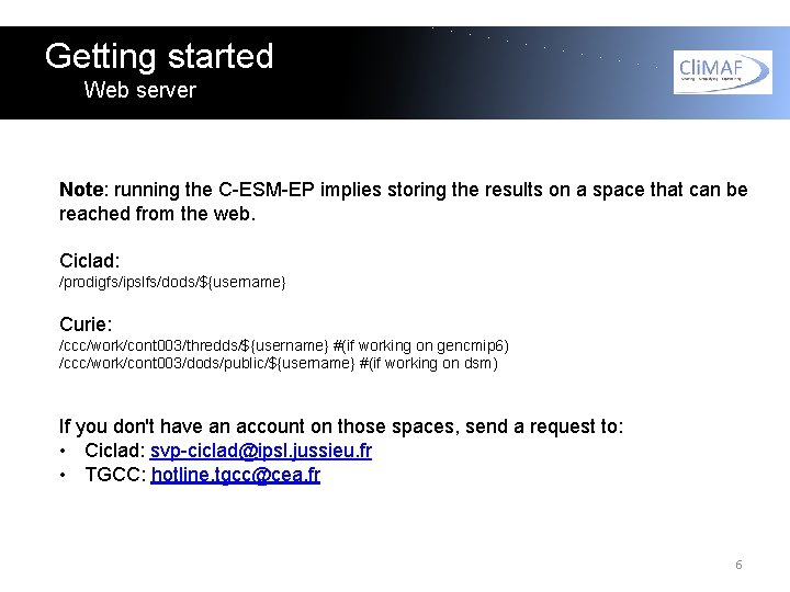
Getting started Web server Note: running the C-ESM-EP implies storing the results on a space that can be reached from the web. Ciclad: /prodigfs/ipslfs/dods/${username} Curie: /ccc/work/cont 003/thredds/${username} #(if working on gencmip 6) /ccc/work/cont 003/dods/public/${username} #(if working on dsm) If you don't have an account on those spaces, send a request to: • Ciclad: svp-ciclad@ipsl. jussieu. fr • TGCC: hotline. tgcc@cea. fr 6

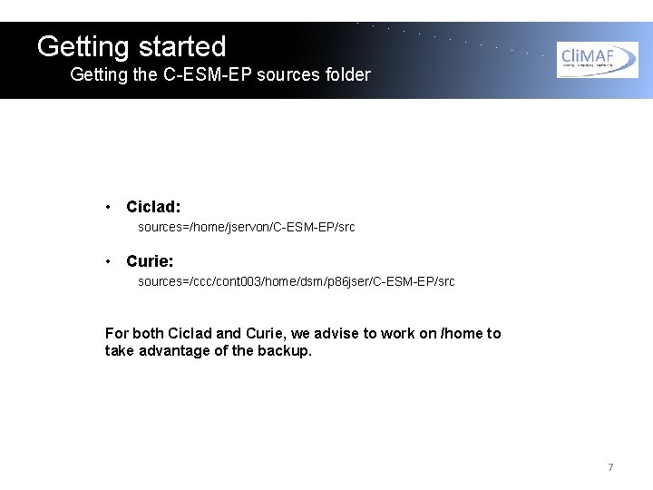
Getting started Getting the C-ESM-EP sources folder • Ciclad: sources=/home/jservon/C-ESM-EP/src • Curie: sources=/ccc/cont 003/home/dsm/p 86 jser/C-ESM-EP/src For both Ciclad and Curie, we advise to work on /home to take advantage of the backup. 7

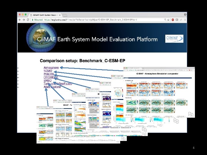
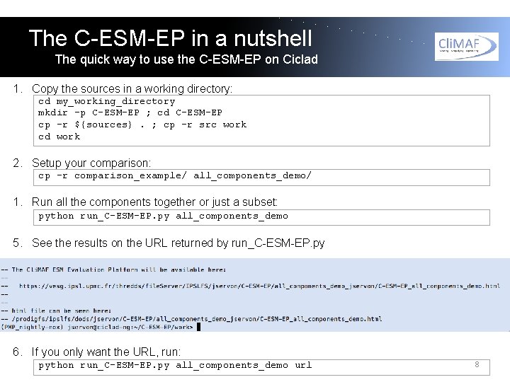
The C-ESM-EP in a nutshell The quick way to use the C-ESM-EP on Ciclad 1. Copy the sources in a working directory: cd my_working_directory mkdir -p C-ESM-EP ; cd C-ESM-EP cp –r ${sources}. ; cp –r src work cd work 2. Setup your comparison: cp -r comparison_example/ all_components_demo/ 1. Run all the components together or just a subset: python run_C-ESM-EP. py all_components_demo 5. See the results on the URL returned by run_C-ESM-EP. py 6. If you only want the URL, run: python run_C-ESM-EP. py all_components_demo url 8

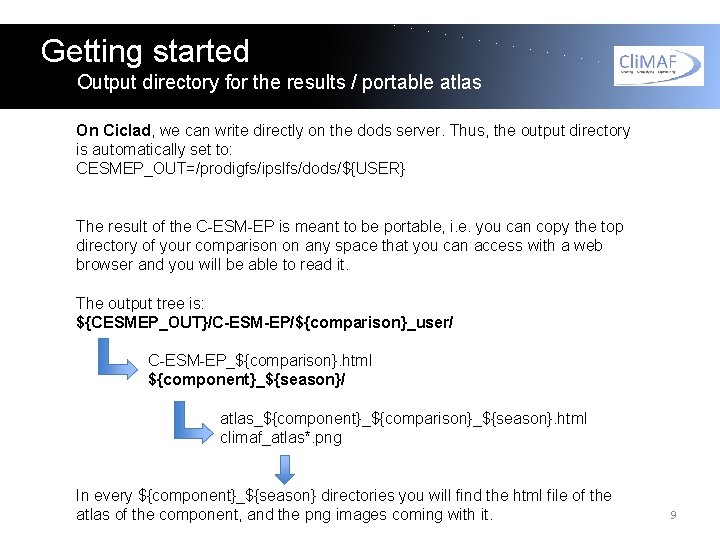
Getting started Output directory for the results / portable atlas On Ciclad, we can write directly on the dods server. Thus, the output directory is automatically set to: CESMEP_OUT=/prodigfs/ipslfs/dods/${USER} The result of the C-ESM-EP is meant to be portable, i. e. you can copy the top directory of your comparison on any space that you can access with a web browser and you will be able to read it. The output tree is: ${CESMEP_OUT}/C-ESM-EP/${comparison}_user/ C-ESM-EP_${comparison}. html ${component}_${season}/ atlas_${component}_${comparison}_${season}. html climaf_atlas*. png In every ${component}_${season} directories you will find the html file of the atlas of the component, and the png images coming with it. 9

2. Playing with Atlas Explorer 10

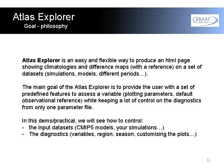
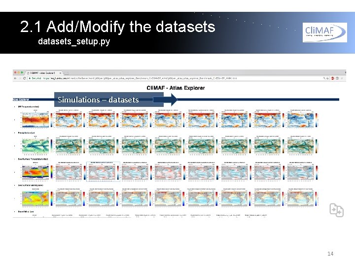
Atlas Explorer Goal - philosophy Atlas Explorer is an easy and flexible way to produce an html page showing climatologies and difference maps (with a reference) on a set of datasets (simulations, models, different periods…). The main goal of the Atlas Explorer is to provide the user with a set of predefined features to assess a variable (plotting parameters, default observational reference) while keeping a lot of control on the diagnostics from only one parameter file. In this demo/practical, we will see how to control: - the input datasets (CMIP 5 models, your simulations…) - The diagnostics (variables, region, season, customising the plots…) 11

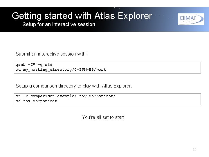
Getting started with Atlas Explorer Setup for an interactive session Submit an interactive session with: qsub –IV –q std cd my_working_directory/C-ESM-EP/work Setup a comparison directory to play with Atlas Explorer: cp -r comparison_example/ toy_comparison/ cd toy_comparison You're all set to start! 12

2. 1 Add/modify datasets 13

2. 1 Add/Modify the datasets_setup. py Simulations – datasets 14

2. 1 Add/Modify the datasets_setup. py The datasets are specified in datasets_setup. py The datasets are defined as python dictionaries containing the keywords/values pairs that are typically used by the Cli. MAF function ds() to access the data (but the variable). The dictionaries can contain some custom control on the diagnostics (provide a season, a period and frequency specific to a diagnostic…). Let's start by opening datasets_setup. py with your favourite editor: vi datasets_setup. py We will now learn how to add or modify the datasets in datasets_setup. py, using the pre-existing Cli. MAF projects (data access definitions). 15

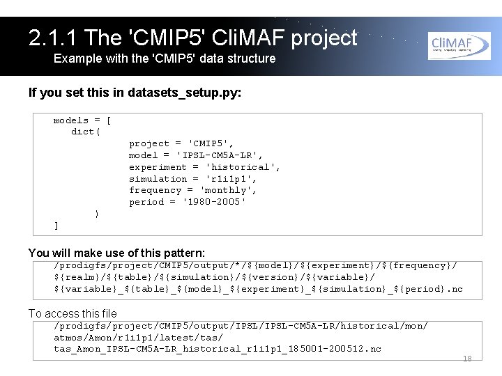
2. 1. 1 Cli. MAF datasets Standardized interface to access datasets Cli. MAF provides a standardized way to access different data structures, defined with Cli. MAF projects, with a set of common/mandatory keys and possible specific keys to describe the data structure. We access the datasets with the function ds() (shortcut to cdataset()) by providing pairs of keywords/values. Example (in Cli. MAF code): dat = ds( project = 'CMIP 5', model = 'IPSL-CM 5 A-LR', experiment = 'historical', simulation = 'r 1 i 1 p 1', variable = 'tas', frequency = 'monthly', period = '1980 -2005' ) Mandatory / specific This functionality allows defining variable name aliases (potential scale/offset), so that you can work on all the different data structures with CMIP variables names and SI units. 16

2. 1. 1 The Cli. MAF projects Getting access to the various data structures In Cli. MAF, we get access to the datasets through Cli. MAF 'projects'. A Cli. MAF project is defined by: - a pattern to access the data - a set of keywords that define the dataset (path + filename + variable) - a set of aliases (variables and frequency) between the names in the files and the CMIP standard names Have a look at the documentation here: http: //climaf. readthedocs. io/en/latest/functions_data. html? highlight=cproject And/or look at the examples (projects already defined in Cli. MAF) in the Cli. MAF version used for the C-ESM-EP: /home/jservon/Evaluation/Cli. MAF/climaf_installs/climaf_1. 0. 3_CESMEP/cli maf/projects The igcm_out. py project file is a good example. 17

2. 1. 1 The 'CMIP 5' Cli. MAF project Example with the 'CMIP 5' data structure If you set this in datasets_setup. py: models = [ dict( project = 'CMIP 5', model = 'IPSL-CM 5 A-LR', experiment = 'historical', simulation = 'r 1 i 1 p 1', frequency = 'monthly', period = '1980 -2005' ) ] You will make use of this pattern: /prodigfs/project/CMIP 5/output/*/${model}/${experiment}/${frequency}/ ${realm}/${table}/${simulation}/${version}/${variable}/ ${variable}_${table}_${model}_${experiment}_${simulation}_${period}. nc To access this file /prodigfs/project/CMIP 5/output/IPSL-CM 5 A-LR/historical/mon/ atmos/Amon/r 1 i 1 p 1/latest/tas/ tas_Amon_IPSL-CM 5 A-LR_historical_r 1 i 1 p 1_185001 -200512. nc 18

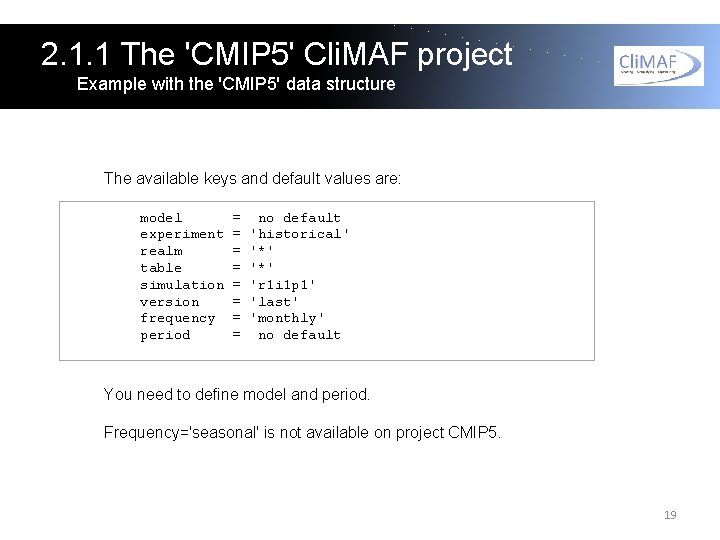
2. 1. 1 The 'CMIP 5' Cli. MAF project Example with the 'CMIP 5' data structure The available keys and default values are: model experiment realm table simulation version frequency period = = = = no default 'historical' '*' 'r 1 i 1 p 1' 'last' 'monthly' no default You need to define model and period. Frequency='seasonal' is not available on project CMIP 5. 19

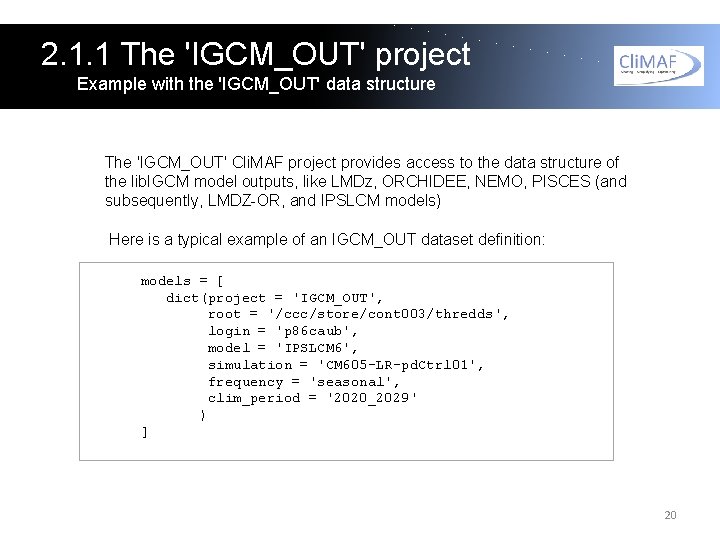
2. 1. 1 The 'IGCM_OUT' project Example with the 'IGCM_OUT' data structure The 'IGCM_OUT' Cli. MAF project provides access to the data structure of the lib. IGCM model outputs, like LMDz, ORCHIDEE, NEMO, PISCES (and subsequently, LMDZ-OR, and IPSLCM models) Here is a typical example of an IGCM_OUT dataset definition: models = [ dict(project = 'IGCM_OUT', root = '/ccc/store/cont 003/thredds', login = 'p 86 caub', model = 'IPSLCM 6', simulation = 'CM 605 -LR-pd. Ctrl 01', frequency = 'seasonal', clim_period = '2020_2029' ) ] 20

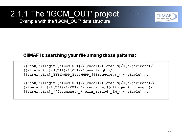
2. 1. 1 The 'IGCM_OUT' project Example with the 'IGCM_OUT' data structure Cli. MAF is searching your file among those patterns: ${root}/${login}[/IGCM_OUT]/${model}/${status}/${experiment}/ ${simulation}/${DIR}/${OUT}/${ave_length}/ ${simulation}_YYYYMMDD_${frequency}_${variable}. nc ${root}/${login}[/IGCM_OUT]/${model}/${status}/${experiment}/$ {simulation}/${DIR}/${OUT}/${frequency}${clim_period_length}/ ${simulation}_${frequency}_${clim_period}_1 M_${variable}. nc 21

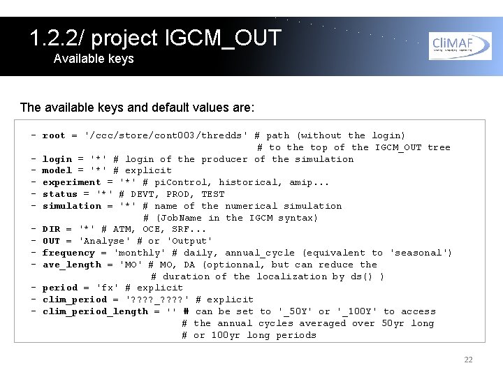
1. 2. 2/ project IGCM_OUT Available keys The available keys and default values are: - root = '/ccc/store/cont 003/thredds' # path (without the login) # to the top of the IGCM_OUT tree - login = '*' # login of the producer of the simulation - model = '*' # explicit - experiment = '*' # pi. Control, historical, amip. . . - status = '*' # DEVT, PROD, TEST - simulation = '*' # name of the numerical simulation # (Job. Name in the IGCM syntax) - DIR = '*' # ATM, OCE, SRF. . . - OUT = 'Analyse' # or 'Output' - frequency = 'monthly' # daily, annual_cycle (equivalent to 'seasonal') - ave_length = 'MO' # MO, DA (optionnal, but can reduce the # duration of the localization by ds() ) - period = 'fx' # explicit - clim_period = '? ? _? ? ' # explicit - clim_period_length = '' # can be set to '_50 Y' or '_100 Y' to access # the annual cycles averaged over 50 yr long # or 100 yr long periods 22

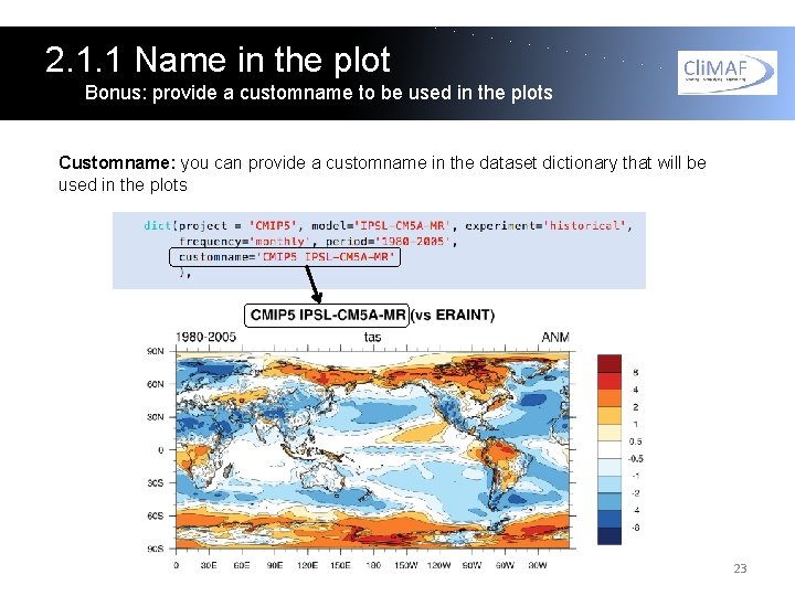
2. 1. 1 Name in the plot Bonus: provide a customname to be used in the plots Customname: you can provide a customname in the dataset dictionary that will be used in the plots 23

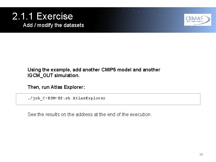
2. 1. 1 Exercise Add / modify the datasets Using the example, add another CMIP 5 model and another IGCM_OUT simulation. Then, run Atlas Explorer: . /job_C-ESM-EP. sh Atlas. Explorer See the results on the address at the end of the execution. 24

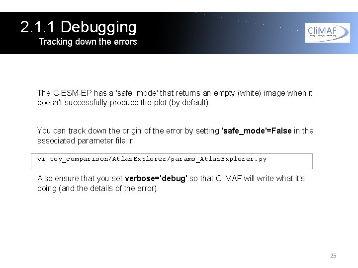
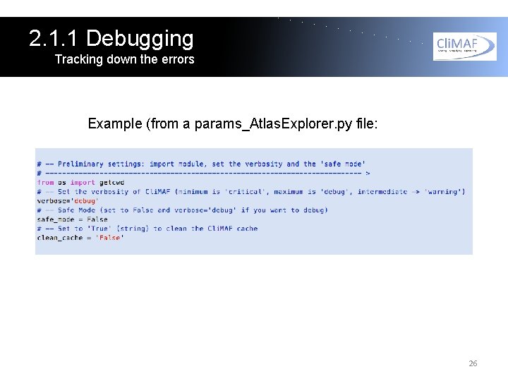
2. 1. 1 Debugging Tracking down the errors The C-ESM-EP has a 'safe_mode' that returns an empty (white) image when it doesn't successfully produce the plot (by default). You can track down the origin of the error by setting 'safe_mode'=False in the associated parameter file in: vi toy_comparison/Atlas. Explorer/params_Atlas. Explorer. py Also ensure that you set verbose='debug' so that Cli. MAF will write what it's doing (and the details of the error). 25

2. 1. 1 Debugging Tracking down the errors Example (from a params_Atlas. Explorer. py file: 26

2. 1. 2 Control the period Period selection in brief in CMIP 5 and IGCM_OUT The C-ESM-EP essentially works on 'monthly' and 'seasonal' datasets. With the 'monthly' datasets, Cli. MAF can perform a smart period selection on the available netcdf files. With the 'seasonal' datasets, Cli. MAF only selects an existing seasonal cycle netcdf file. The C-ESM-EP, however, has a smart way to select the last/first seasonal cycle available. Both CMIP 5 and IGCM_OUT projects have monthly datasets. Only IGCM_OUT (and the ref_climatos project) provides seasonal datasets. 27

2. 1. 2 Control the period Period selection in the CMIP 5 project One of the great features of Cli. MAF is the automatic selection of the period provided by the user. When you set frequency='monthly', you have to provide a period that will be extracted among the non-overlapping netcdf files in the targeted directory. For instance, this dataset definition: dict(project = 'CMIP 5', model = 'IPSL-CM 5 A-LR', experiment = 'historical', simulation = 'r 1 i 1 p 1', frequency = 'monthly', period = '1980 -2005') Will extract the period 1980 -2005 from this file found in the archive: /prodigfs/project/CMIP 5/output/IPSL-CM 5 ALR/historical/mon/atmos/Amon/r 1 i 1 p 1/latest/tas/ tas_Amon_IPSL-CM 5 A-LR_historical_r 1 i 1 p 1_185001 -200512. nc 28

2. 1. 2 Control the period and frequency Period selection in IGCM_OUT In the IGCM_OUT project, you will have the same behaviour as for the CMIP 5 project with frequency='monthly' (fundamental Cli. MAF functionality). By default, it will target the 'TS_MO' time series files created by the postprocessing (one variable per file with all time steps). If you want to get the data from the 'Output/MO' files, add OUT='Output' to the list of arguments : dict(project = 'IGCM_OUT', root = '/ccc/store/cont 003/thredds', login = 'p 86 caub', model = 'IPSLCM 6', simulation = 'CM 605 -LR-pd. Ctrl 01' frequency = 'monthly', OUT='Output', period = '2020_2029') 29

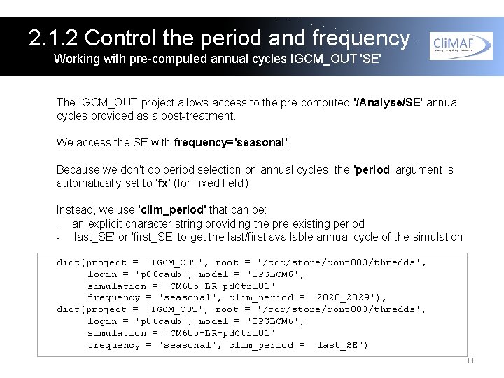
2. 1. 2 Control the period and frequency Working with pre-computed annual cycles IGCM_OUT 'SE' The IGCM_OUT project allows access to the pre-computed '/Analyse/SE' annual cycles provided as a post-treatment. We access the SE with frequency='seasonal'. Because we don't do period selection on annual cycles, the 'period' argument is automatically set to 'fx' (for 'fixed field'). Instead, we use 'clim_period' that can be: - an explicit character string providing the pre-existing period - 'last_SE' or 'first_SE' to get the last/first available annual cycle of the simulation dict(project = 'IGCM_OUT', root = '/ccc/store/cont 003/thredds', login = 'p 86 caub', model = 'IPSLCM 6', simulation = 'CM 605 -LR-pd. Ctrl 01' frequency = 'seasonal', clim_period = '2020_2029'), dict(project = 'IGCM_OUT', root = '/ccc/store/cont 003/thredds', login = 'p 86 caub', model = 'IPSLCM 6', simulation = 'CM 605 -LR-pd. Ctrl 01' frequency = 'seasonal', clim_period = 'last_SE') 30

2. 1. 2 clim_period and ts_period Period for the clim. and the time series C-ESM-EP diagnostics The C-ESM-EP is composed of 'climatology diagnostics' (like bias maps) and 'time series diagnostics' (like the AMOC index or ENSO diagnostics). Because of this, the user might want to provide one period for the climatologies, and one for the time series. The diagnostics of the Atlas Explorer are only 'climatology diagnostics'. We will describe how to handle the 'time series diagnostics' also here, but it will not be applicable to the Atlas Explorer. 31

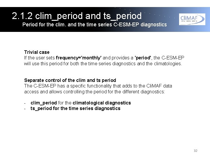
2. 1. 2 clim_period and ts_period Period for the clim. and the time series C-ESM-EP diagnostics Trivial case If the user sets frequency='monthly' and provides a 'period', the C-ESM-EP will use this period for both the time series diagnostics and the climatologies. Separate control of the clim and ts period The C-ESM-EP has a specific functionality that adds to the Cli. MAF data access and allows controlling the period for the different diagnostics: - clim_period for the climatological diagnostics ts_period for the time series diagnostics 32

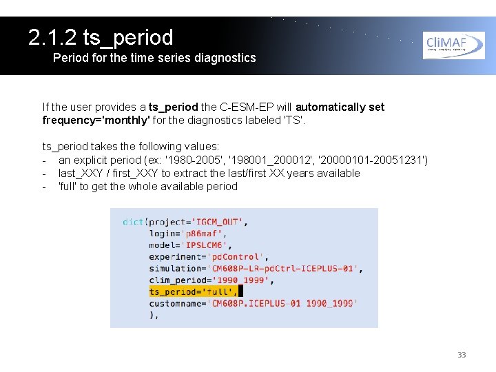
2. 1. 2 ts_period Period for the time series diagnostics If the user provides a ts_period the C-ESM-EP will automatically set frequency='monthly' for the diagnostics labeled 'TS'. ts_period takes the following values: - an explicit period (ex: '1980 -2005', '198001_200012', '20000101 -20051231') - last_XXY / first_XXY to extract the last/first XX years available - 'full' to get the whole available period 33

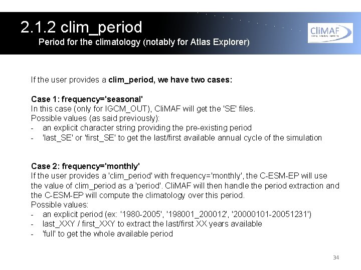
2. 1. 2 clim_period Period for the climatology (notably for Atlas Explorer) If the user provides a clim_period, we have two cases: Case 1: frequency='seasonal' In this case (only for IGCM_OUT), Cli. MAF will get the 'SE' files. Possible values (as said previously): - an explicit character string providing the pre-existing period - 'last_SE' or 'first_SE' to get the last/first available annual cycle of the simulation Case 2: frequency='monthly' If the user provides a 'clim_period' with frequency='monthly', the C-ESM-EP will use the value of clim_period as a 'period'. Cli. MAF will then handle the period extraction and the C-ESM-EP will compute the climatology over this period. Possible values: - an explicit period (ex: '1980 -2005', '198001_200012', '20000101 -20051231') - last_XXY / first_XXY to extract the last/first XX years available - 'full' to get the whole available period 34

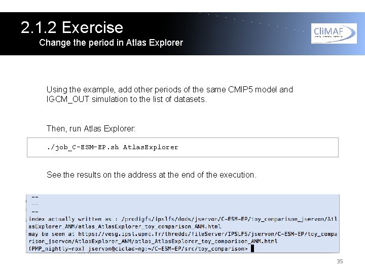
2. 1. 2 Exercise Change the period in Atlas Explorer Using the example, add other periods of the same CMIP 5 model and IGCM_OUT simulation to the list of datasets. Then, run Atlas Explorer: . /job_C-ESM-EP. sh Atlas. Explorer See the results on the address at the end of the execution. 35

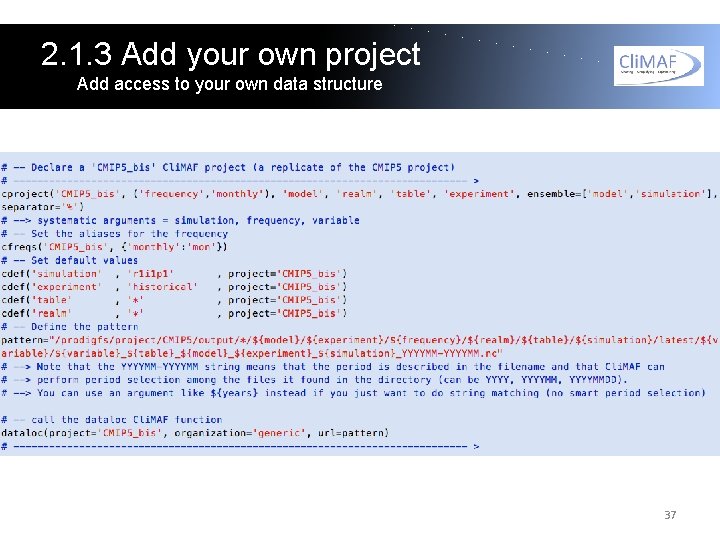
2. 1. 3 Add your own project Access your own datasets You can easily access your own datasets by creating a Cli. MAF project directly in datasets_setup. py. You will find an example in datasets_setup. py with a 'CMIP 5_bis' project (same as next slide). The minimum you have to do is a 'cproject' and a 'dataloc'. You will also see how to use cdef() (define default values) and cfreqs() (aliases for the frequency names). You're also invited to look at the Cli. MAF documentation for the use of those functions, and get some inspiration from the Cli. MAF projects in: /home/jservon/Evaluation/Cli. MAF/climaf_installs/climaf_1. 0. 3_C ESMEP/climaf/projects 36

2. 1. 3 Add your own project Add access to your own data structure 37

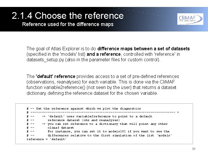
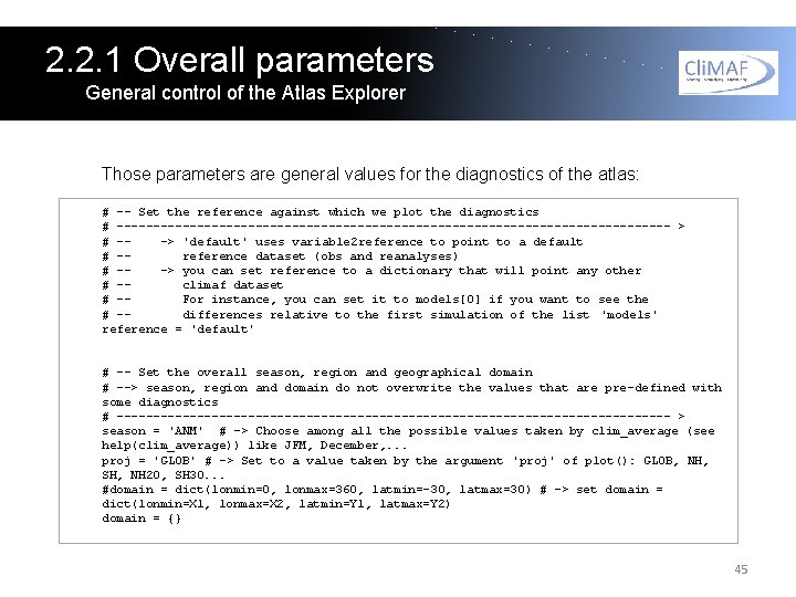
2. 1. 4 Choose the reference Reference used for the difference maps The goal of Atlas Explorer is to do difference maps between a set of datasets (specified in the 'models' list) and a reference, controlled with 'reference' in datasets_setup. py (also in the parameter files for custom control). The 'default' reference provides access to a set of pre-defined references (observations, reanalyses) for each variable. This is done via the Cli. MAF function variable 2 reference() (not seen by the user) that returns a dataset dictionary defining the reference dataset for the chosen variable. # -- Set the reference against which we plot the diagnostics # -------------------------------------- > # --> 'default' uses variable 2 reference to point to a default # -reference dataset (obs and reanalyses) # --> you can set reference to a dictionary that will point any other # -climaf dataset # -For instance, you can set it to models[0] if you want to see the # -differences relative to the first simulation of the list 'models' reference = 'default' 38

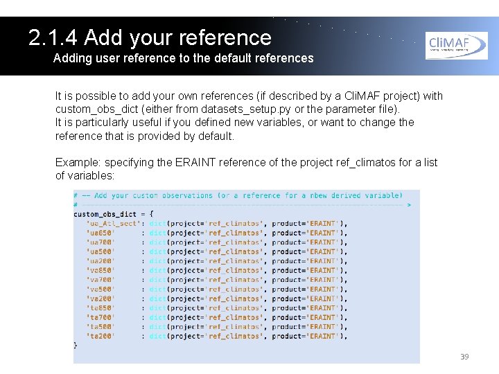
2. 1. 4 Add your reference Adding user reference to the default references It is possible to add your own references (if described by a Cli. MAF project) with custom_obs_dict (either from datasets_setup. py or the parameter file). It is particularly useful if you defined new variables, or want to change the reference that is provided by default. Example: specifying the ERAINT reference of the project ref_climatos for a list of variables: 39

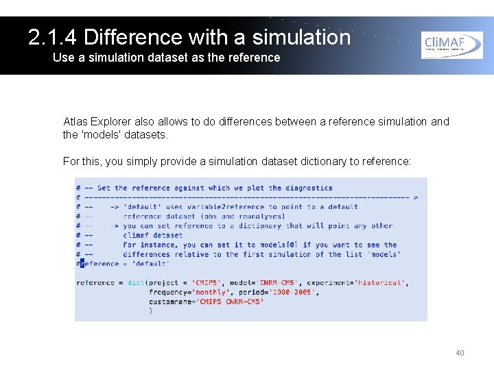
2. 1. 4 Difference with a simulation Use a simulation dataset as the reference Atlas Explorer also allows to do differences between a reference simulation and the 'models' datasets. For this, you simply provide a simulation dataset dictionary to reference: 40

2. 1. 4 Difference with a simulation Use a simulation dataset as the reference Note 1 Cli. MAF offers a set of pre-defined plot parameters, depending on the 'context': full_field (for a climatology), 'bias', and 'model_model' for model-model differences. The C-ESM-EP automatically defines the context by analysing the input datasets. In that case, Cli. MAF will use the pre-defined plot parameters for the 'model_model' differences (and not the 'bias' differences). (more details in section 2. 2. 4) Note 2 Much of our climate science consists in doing climatologies and differences…This functionality provides a huge amount of possibilities: - Differences of targeted periods of a simulation relative to the climatology of this simulation - Evolution of a simulation relative to the first month/year - Differences of a set of simulations with a reference model version - … 41

2. 2 Atlas. Explorer parameter file 42

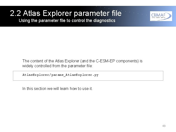
2. 2 Atlas Explorer parameter file Using the parameter file to control the diagnostics The content of the Atlas Explorer (and the C-ESM-EP components) is widely controlled from the parameter file: Atlas. Explorer/params_Atlas. Explorer. py In this section we will learn how to use it. 43

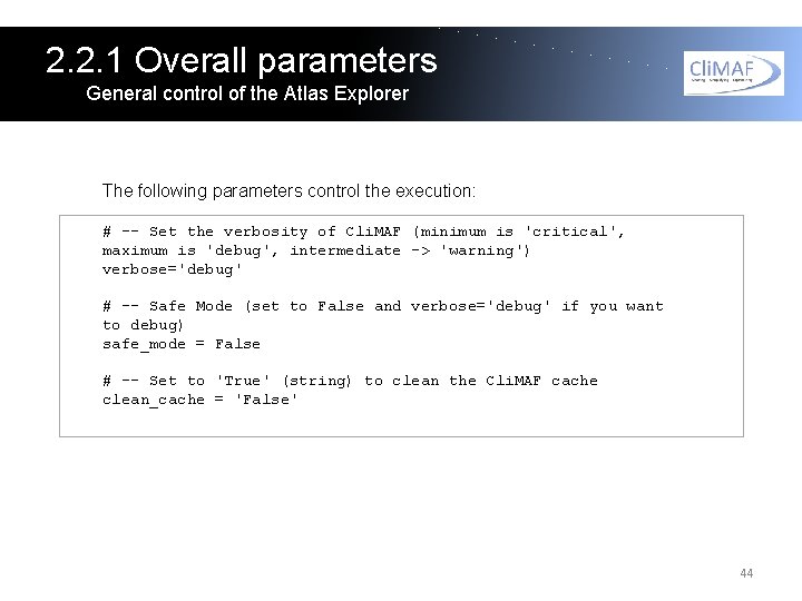
2. 2. 1 Overall parameters General control of the Atlas Explorer The following parameters control the execution: # -- Set the verbosity of Cli. MAF (minimum is 'critical', maximum is 'debug', intermediate -> 'warning') verbose='debug' # -- Safe Mode (set to False and verbose='debug' if you want to debug) safe_mode = False # -- Set to 'True' (string) to clean the Cli. MAF cache clean_cache = 'False' 44

2. 2. 1 Overall parameters General control of the Atlas Explorer Those parameters are general values for the diagnostics of the atlas: # -- Set the reference against which we plot the diagnostics # -------------------------------------- > # --> 'default' uses variable 2 reference to point to a default # -reference dataset (obs and reanalyses) # --> you can set reference to a dictionary that will point any other # -climaf dataset # -For instance, you can set it to models[0] if you want to see the # -differences relative to the first simulation of the list 'models' reference = 'default' # -- Set the overall season, region and geographical domain # --> season, region and domain do not overwrite the values that are pre-defined with some diagnostics # -------------------------------------- > season = 'ANM' # -> Choose among all the possible values taken by clim_average (see help(clim_average)) like JFM, December, . . . proj = 'GLOB' # -> Set to a value taken by the argument 'proj' of plot(): GLOB, NH, SH, NH 20, SH 30. . . #domain = dict(lonmin=0, lonmax=360, latmin=-30, latmax=30) # -> set domain = dict(lonmin=X 1, lonmax=X 2, latmin=Y 1, latmax=Y 2) domain = {} 45

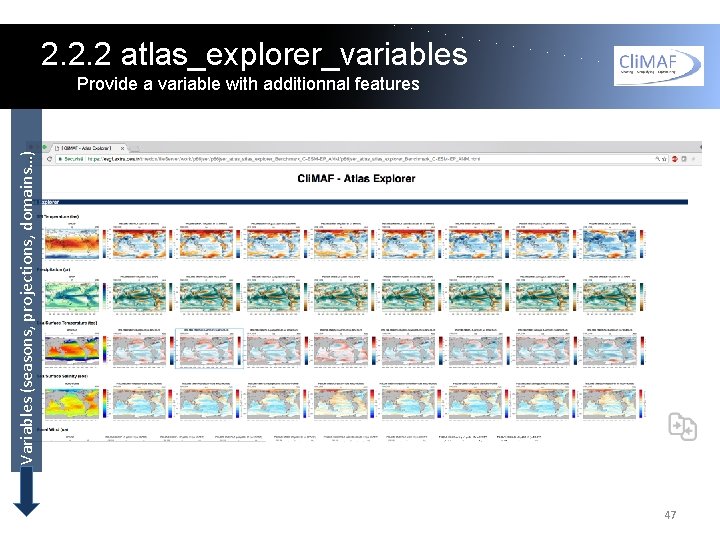
2. 2. 2 atlas_explorer_variables Provide a variable with additionnal features One of the goals of Atlas Explorer is to provide the user with an easy control of the scientific content of the atlas. Each line of the html page is an element of the atlas_explorer_variables list in the params_Atlas. Explorer. py file. 46

2. 2. 2 atlas_explorer_variables Variables (seasons, projections, domains…) Provide a variable with additionnal features 47

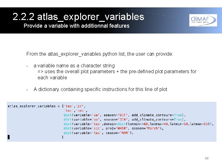
2. 2. 2 atlas_explorer_variables Provide a variable with additionnal features From the atlas_explorer_variables python list, the user can provide: - a variable name as a character string => uses the overall plot parameters + the pre-defined plot parameters for each variable - A dictionary containing specific instructions for this line of plot 48

2. 2. 2 atlas_explorer_variables Provide a variable with additionnal features Here is the list of arguments that you can control from the dictionary of a variable: All arguments that the 'plot' Cli. MAF function can take: - http: //climaf. readthedocs. io/en/latest/scripts/plot. html - proj: the projection used (GLOB, NH 20, SH 60…) - contours: add contours - colors, min, max, delta: control the color isolines - color: an NCL color palette - … See next slide 49

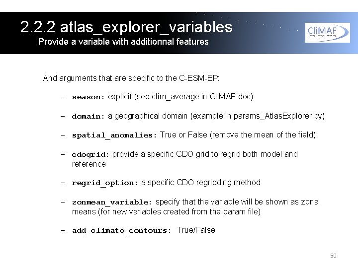
2. 2. 2 atlas_explorer_variables Provide a variable with additionnal features And arguments that are specific to the C-ESM-EP: - season: explicit (see clim_average in Cli. MAF doc) - domain: a geographical domain (example in params_Atlas. Explorer. py) - spatial_anomalies: True or False (remove the mean of the field) - cdogrid: provide a specific CDO grid to regrid both model and reference - regrid_option: a specific CDO regridding method - zonmean_variable: specify that the variable will be shown as zonal means (for new variables created from the param file) - add_climato_contours: True/False 50

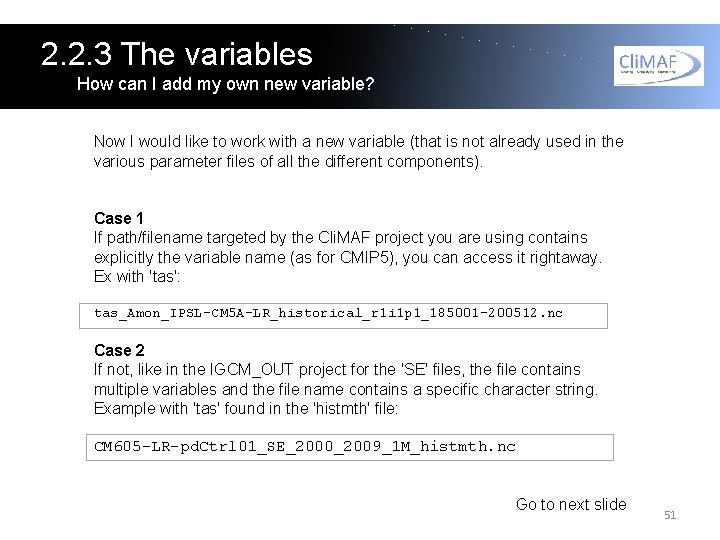
2. 2. 3 The variables How can I add my own new variable? Now I would like to work with a new variable (that is not already used in the various parameter files of all the different components). Case 1 If path/filename targeted by the Cli. MAF project you are using contains explicitly the variable name (as for CMIP 5), you can access it rightaway. Ex with 'tas': tas_Amon_IPSL-CM 5 A-LR_historical_r 1 i 1 p 1_185001 -200512. nc Case 2 If not, like in the IGCM_OUT project for the 'SE' files, the file contains multiple variables and the file name contains a specific character string. Example with 'tas' found in the 'histmth' file: CM 605 -LR-pd. Ctrl 01_SE_2000_2009_1 M_histmth. nc Go to next slide 51

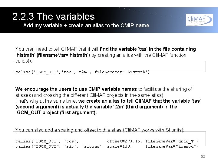
2. 2. 3 The variables Add my variable + create an alias to the CMIP name You then need to tell Cli. MAF that it will find the variable 'tas' in the file containing 'histmth' (filename. Var='histmth') by creating an alias with the Cli. MAF function calias(): calias('IGCM_OUT', 'tas', 't 2 m', filename. Var='histmth') We encourage the users to use CMIP variable names to facilitate the sharing of atlases (and crossing the different Cli. MAF projects in the same atlas). That's why at the same time, we create an alias to tell Cli. MAF that the variable 'tas' (second argument) is actually the variable 't 2 m' (third argument) in the IGCM_OUT project (first argument). You can also add a scaling and offset to this alias (Cli. MAF works with SI units): calias("IGCM_OUT", 'tos', offset=273. 15, filename. Var='grid_T') calias("IGCM_OUT", 'sic', 'siconc', scale=100, filename. Var="icemod") 52

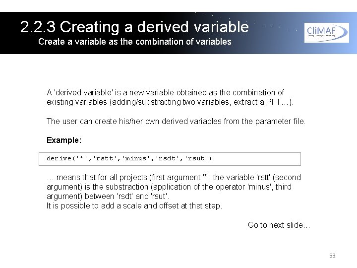
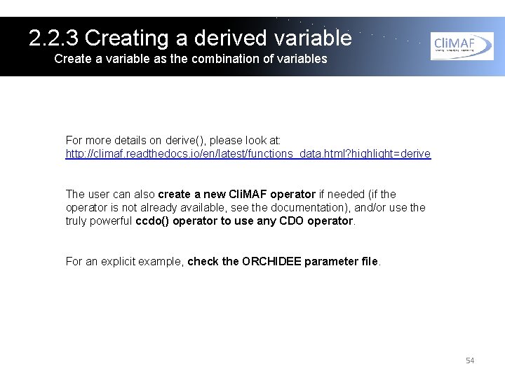
2. 2. 3 Creating a derived variable Create a variable as the combination of variables A 'derived variable' is a new variable obtained as the combination of existing variables (adding/substracting two variables, extract a PFT…). The user can create his/her own derived variables from the parameter file. Example: derive('*', 'rstt', 'minus', 'rsdt', 'rsut') … means that for all projects (first argument '*', the variable 'rstt' (second argument) is the substraction (application of the operator 'minus', third argument) between 'rsdt' and 'rsut'. It is possible to add a scale and offset at that step. Go to next slide… 53

2. 2. 3 Creating a derived variable Create a variable as the combination of variables For more details on derive(), please look at: http: //climaf. readthedocs. io/en/latest/functions_data. html? highlight=derive The user can also create a new Cli. MAF operator if needed (if the operator is not already available, see the documentation), and/or use the truly powerful ccdo() operator to use any CDO operator. For an explicit example, check the ORCHIDEE parameter file. 54

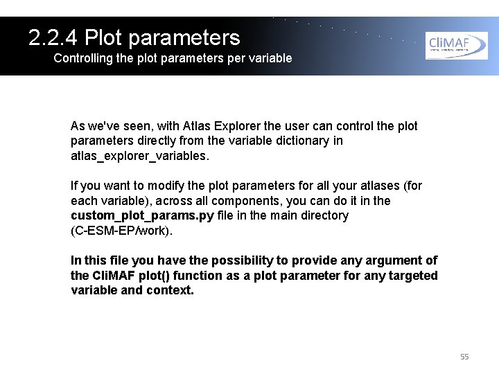
2. 2. 4 Plot parameters Controlling the plot parameters per variable As we've seen, with Atlas Explorer the user can control the plot parameters directly from the variable dictionary in atlas_explorer_variables. If you want to modify the plot parameters for all your atlases (for each variable), across all components, you can do it in the custom_plot_params. py file in the main directory (C-ESM-EP/work). In this file you have the possibility to provide any argument of the Cli. MAF plot() function as a plot parameter for any targeted variable and context. 55

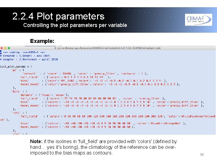
2. 2. 4 Plot parameters Controlling the plot parameters per variable Example: Note: if the isolines in 'full_field' are provided with 'colors' (defined by hand… yes it's boring), the climatology of the reference can be overimposed to the bias maps as contours. 56

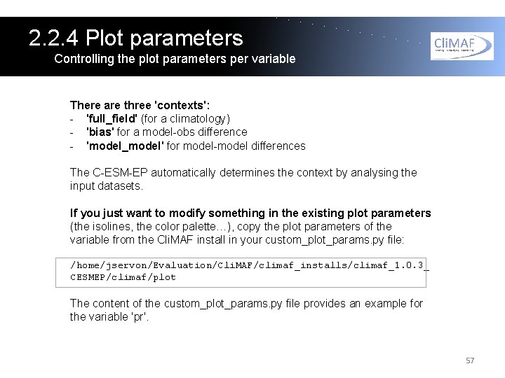
2. 2. 4 Plot parameters Controlling the plot parameters per variable There are three 'contexts': - 'full_field' (for a climatology) - 'bias' for a model-obs difference - 'model_model' for model-model differences The C-ESM-EP automatically determines the context by analysing the input datasets. If you just want to modify something in the existing plot parameters (the isolines, the color palette…), copy the plot parameters of the variable from the Cli. MAF install in your custom_plot_params. py file: /home/jservon/Evaluation/Cli. MAF/climaf_installs/climaf_1. 0. 3_ CESMEP/climaf/plot The content of the custom_plot_params. py file provides an example for the variable 'pr'. 57

The compare. Companion 58

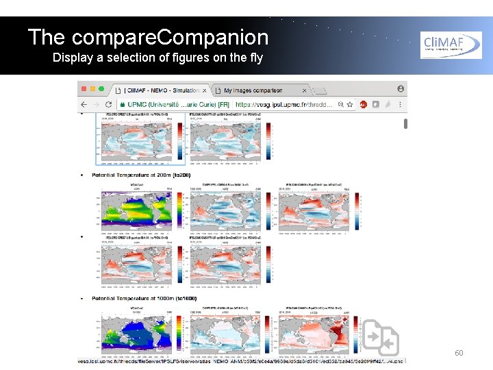
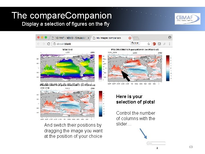
The compare. Companion Display a selection of figures on the fly The various html pages can provide a lot of information and you might need to select a subset of them to focus on a particular question. For this, the C-ESM-EP comes with an 'on-the-fly' tool to select a subset of plots, called the compare. Companion (P. Brockmann). 59

The compare. Companion Display a selection of figures on the fly 60

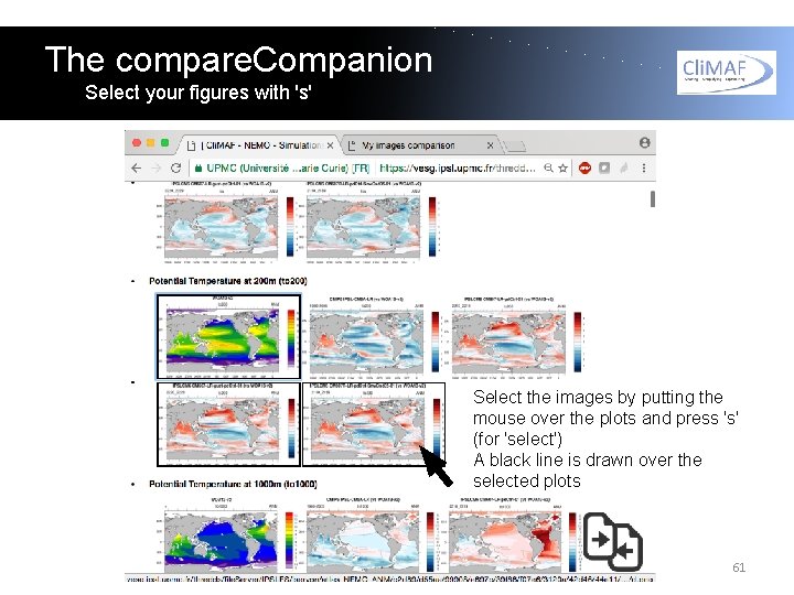
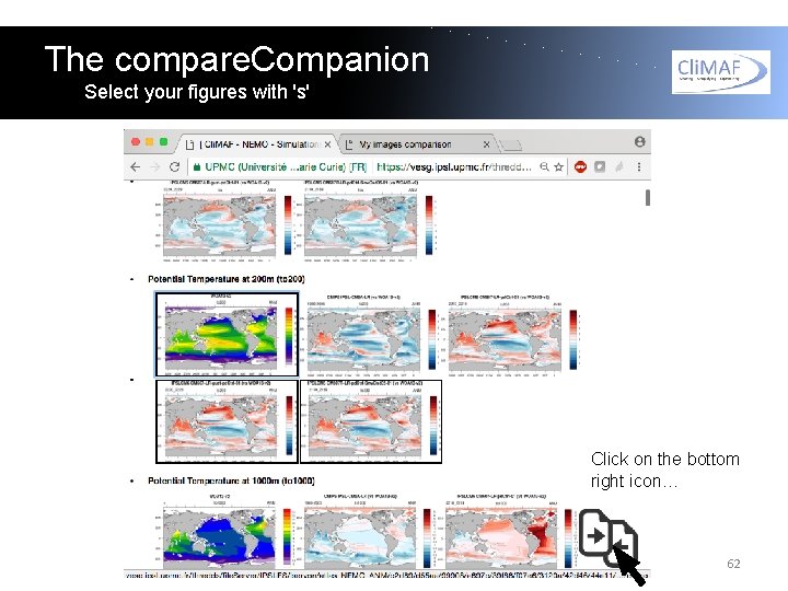
The compare. Companion Select your figures with 's' Select the images by putting the mouse over the plots and press 's' (for 'select') A black line is drawn over the selected plots 61

The compare. Companion Select your figures with 's' Click on the bottom right icon… 62

The compare. Companion Display a selection of figures on the fly Here is your selection of plots! And switch their positions by dragging the image you want at the position of your choice Control the number of columns with the slider… 63

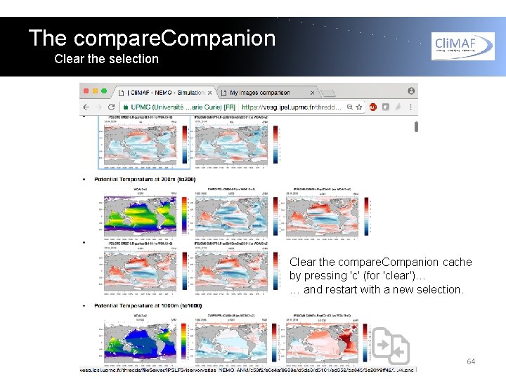
The compare. Companion Clear the selection Clear the compare. Companion cache by pressing 'c' (for 'clear')… … and restart with a new selection. 64

Questions? jerome. servonnat@lsce. ipsl. fr 65

The Cli. MAF Earth System Model Evaluation Platform, 2017 J. Servonnat, S. Sénési, L. Vignon, O. Marti, P. Brockmann, S. Denvil Contributors: F. Hourdin, I. Musat, M. P. Moine, E. Sanchez, M. Chevallier, R. Msadek, J. Deshayes, M. Van Coppenolle, C. Rousset, J. Mignot, J. Ghattas, P. Peylin, N. Vuichard, P. Cadule, A. Ducharne, F. Maignan, R. Séférian Beta-testers: O. Marti, J. Mignot, J. Deshayes, P. Braconnot, P. Sepulchre, M. Kageyama, S. Denvil, R. Séférian, A. Cozic The authors would like to give special credit to A. Voldoire for showing the way for Cli. MAF, and to F. Hourdin and the LMDz team for the structure of the CESM-EP that is largely inspired from the LMDz evaluation atlas. 66