Classification with Decision Trees and Rules Density Estimation

Classification with Decision Trees and Rules

Density Estimation – looking ahead • Compare it against the two other major kinds of models: Input Attributes Classifier Prediction of categorical output or class One of a few discrete values Input Attributes Copyright © Andrew W. Moore Density Estimator Probability Regresso r Prediction of real-valued output

DECISION TREE LEARNING: OVERVIEW

Decision tree learning

A decision tree

Another format: a set of rules if O=sunny and H<= 70 then PLAY else if O=sunny and H>70 then DON’T_PLAY else if O=overcast then PLAY else if O=rain and windy then DON’T_PLAY One rule per leaf in the tree else if O=rain and !windy then PLAY Simpler rule set if O=sunny and H> 70 then DON’T_PLAY else if O=rain and windy then DON’T_PLAY else PLAY

A regression tree Play ~= 33 Play ~= 24 Play ~= 18 Play ~= 48 Play = 45 m, 45, 60, 40 Play ~= 37 Play = 30 m, 45 min Play ~= 5 Play = 0 m, 15 m Play ~= 0 Play = 0 m, 0 m Play ~= 32 Play = 20 m, 30 m,

Motivations for trees and rules • Often you can find a fairly accurate classifier which is small and easy to understand. – Sometimes this gives you useful insight into a problem, or helps you debug a feature set. • Sometimes features interact in complicated ways – Trees can find interactions (e. g. , “sunny and humid”). Again, sometimes this gives you some insight into the problem. • Trees are very inexpensive at test time – You don’t always even need to compute all the features of an example. – You can even build classifiers that take this into account…. – Sometimes that’s important (e. g. , “blood. Pressure<100” vs “MRIScan=normal” might have different costs to compute).

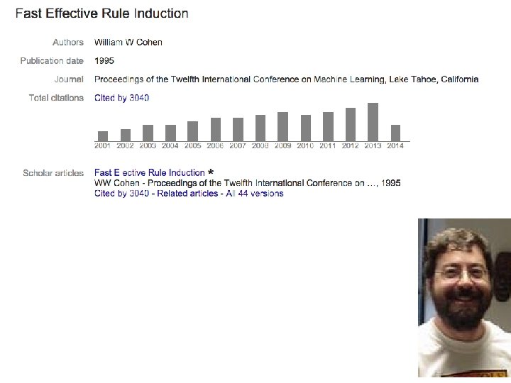
An example: “Is it the Onion”? • On the Onion data… Dataset: 200 Onion articles, ~500 Economist articles. Accuracies: almost 100% with Naïve Bayes! I used a rulelearning method called RIPPER

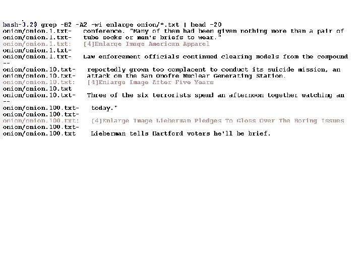
Translation: if “enlarge” is in the set-valued attribute words. Article then class = from. Onion. this rule is correct 173 times, and never wrong … if “added” is in the set-valued attribute words. Article and “play” is in the set-valued attribute words. Article then class = from. Onion. this rule is correct 6 times, and wrong once

After cleaning ‘Enlarge Image’ lines Also, estimated test error rate increases from 1. 4% to 6%

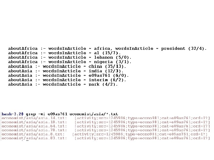
Different Subcategories of Economist Articles

Motivations for trees and rules • Often you can find a fairly accurate classifier which is small and easy to understand. – Sometimes this gives you useful insight into a problem, or helps you debug a feature set. • Sometimes features interact in complicated ways – Trees can find interactions (e. g. , “sunny and humid”) that linear classifiers can’t – Again, sometimes this gives you some insight into the problem. • Trees are very inexpensive at test time – You don’t always even need to compute all the features of an example. – You can even build classifiers that take this into account…. Rest of the class: the algorithms. But – Sometimes that’s important (e. g. , “blood. Pressure<100” vs “MRIScan=normal” have different costs to compute). first…decision might tree learning algorithms are based on information gain heuristics.

BACKGROUND: ENTROPY AND OPTIMAL CODES

Information theory yellow, green, . . . encode 001110… decod e Problem: design an efficient coding scheme for leaf colors: • green • yellow • gold • red • orange • brown yellow, gree n, …

0 5 0. 12 0. 06 0. 25 06 25 5 0. 12 0. 5 1 0 0 01 100 101 1 0 1 1100 1101 111

yellow, green, . . . encode decod e 100 0 … 0 yellow, gree n, … 1 0 0 1 01 0 1 100 101 0 1 1100 1101

0 5 12 0. 25 06 0. 5 0. 12 0. 5 1 0 100 0 01 1 0 1 101 0 1 1100 1101

H p

DECISION TREE LEARNING: THE ALGORITHM(S)

Most decision tree learning algorithms 1. Given dataset D: – return leaf(y) if all examples are in the same class y … or nearly so – pick the best split, on the best attribute a • a=c 1 or a=c 2 or … • a<θ or a ≥ θ • a or not(a) • a in {c 1, …, ck} or not – split the data into D 1 , D 2 , … Dk and recursively build trees for each subset 2. “Prune” the tree

Most decision tree learning algorithms 1. Given dataset D: – return leaf(y) if all examples are in the same class y … or nearly so. . . – pick the best split, on the best attribute a • a=c 1 or a=c 2 or … • a<θ or a ≥ θ • a or not(a) • a in {c 1, …, ck} or not – split the data into D 1 , D 2 , … Dk and recursively build trees for each subset 2. “Prune” the tree Popular splitting criterion: try to lower entropy of the y labels on the resulting partition • i. e. , prefer splits that have skewed distributions of labels

Most decision tree learning algorithms • “Pruning” a tree – avoid overfitting by removing subtrees somehow 15 13 2 11

Most decision tree learning algorithms 1. Given dataset D: – return leaf(y) if all examples are in the same class y … or nearly so. . – pick the best split, on the best attribute a • a<θ or a ≥ θ • a or not(a) • a=c 1 or a=c 2 or … • a in {c 1, …, ck} or not – split the data into D 1 , D 2 , … Dk and recursively build trees for each subset 2. “Prune” the tree 15 Same idea 13

Another view of a decision tree Sepal_length<5. 7 Sepal_width>2. 8

Another view of a decision tree

Another view of a decision tree

Overfitting and k-NN • Small tree a smooth decision boundary • Large tree a complicated shape • What’s the best size decision tree? hi error Error/Loss on an unseen test set Dtest Error/Loss on training set D small tree large tree 31

DECISION TREE LEARNING: BREAKING IT DOWN

Breaking down decision tree learning • First: how to classify - assume everything is binary function pr. Pos = classify. Tree(T, x) if T is a leaf node with counts n, p pr. Pos = (p + 1)/(p + n +2) -- Laplace smoothing else j = T. split. Attribute if x(j)==0 then pr. Pos = classify. Tree(T. left. Son, x) else pr. Pos = classify. Tree(T. right. Son, x)

Breaking down decision tree learning • Reduced error pruning with information gain – Split the data D (2/3, 1/3) into Dgrow and Dprune – Build the tree recursively with Dgrow T = grow. Tree(Dgrow) – Prune the tree with Dprune T’ = prune. Tree(Dprune, T) – Return T’

Breaking down decision tree learning • First: divide & conquer to build the tree with Dgrow function T = grow. Tree(X, Y) if |X|<10 or all. One. Label(Y) then T = leaf. Node(|Y==0|, |Y==1|) -- counts for n, p else for i = 1, …n -- for each attribute i ai = X(: , i) -- column i of X gain(i) = info. Gain( Y, Y(ai==0), Y(ai==1) ) j = argmax(gain); -- the best attribute aj = X(: , j) T = split. Node( grow. Tree(X(aj==0), Y(aj==0)), -- left son grow. Tree(X(aj==1), Y(aj==1)), --right son j)

Breaking down decision tree learning function e = entropy(Y) n = |Y|; p 0 = |Y==0|/n; p 1 = |Y==1| /n; e = - p 0*log(p 0) - p 1*log(p 1)

Breaking down decision tree learning • First: how to build the tree with Dgrow function g = info. Gain(Y, left. Y, right. Y) n = |Y|; n. Left = |left. Y|; n. Right = |right. Y|; g = entropy(Y) - (n. Left/n)*entropy(left. Y) - (n. Right/n)*entropy(right. Y) function e = entropy(Y) n = |Y|; p 0 = |Y==0|/n; p 1 = |Y==1| /n; e = - p 1*log(p 1) - p 2*log(p 2)

Breaking down decision tree learning • Reduced error pruning with information gain – Split the data D (2/3, 1/3) into Dgrow and Dprune – Build the tree recursively with Dgrow T = grow. Tree(Dgrow) – Prune the tree with Dprune T’ = prune. Tree(Dprune) – Return T’

Breaking down decision tree learning • Next: how to prune the tree with Dprune – Estimate the error rate of every subtree on Dprune – Recursively traverse the tree: • Reduce error on the left, right subtrees of T • If T would have lower error if it were converted to a leaf, convert T to a leaf.

We’re using the fact that the examples for sibling subtrees are disjoint. A decision tree

Breaking down decision tree learning • To estimate error rates, classify the whole pruning set, and keep some counts function classify. Prune. Set(T, X, Y) T. prune. N = |Y==0|; T. prune. P = |Y==1| if T is not a leaf then j = T. split. Attribute aj = X(: , j) classify. Prune. Set( T. left. Son, X(aj==0), Y(aj==0) ) classify. Prune. Set( T. right. Son, X(aj==1), Y(aj==1) ) function e = errors. On. Prune. Set. As. Leaf(T): min(T. prune. N, T. prune. P)

Breaking down decision tree learning • Next: how to prune the tree with Dprune – Estimate the error rate of every subtree on Dprune – Recursively traverse the tree: function T 1 = pruned(T) if T is a leaf then -- copy T, adding an error estimate T. min. Errors T 1= leaf(T, errors. On. Prune. Set. As. Leaf(T)) else e 1 = errors. On. Prune. Set. As. Leaf(T) TLeft = pruned(T. left. Son); TRight = pruned(T. right. Son); e 2 = TLeft. min. Errors + TRight. min. Errors; if e 1 <= e 2 then T 1 = leaf(T, e 1) -- cp + add error estimate else T 1 = split. Node(T, e 2) -- cp + add error estimate

Decision trees: plus and minus • Simple and fast to learn • Arguably easy to understand (if compact) • Very fast to use: – often you don’t even need to compute all attribute values • Can find interactions between variables (play if it’s cool and sunny or …. ) and hence nonlinear decision boundaries • Don’t need to worry about how numeric values are scaled

Decision trees: plus and minus • Hard to prove things about • Not well-suited to probabilistic extensions • Sometimes fail badly on problems that seem easy – the IRIS dataset is an example

Fixing decision trees…. • Hard to prove things about • Don’t (typically) improve over linear classifiers when you have lots of features • Sometimes fail badly on problems that linear classifiers perform well on – One solution is to build ensembles of decision trees – more on this later

RULE LEARNING: OVERVIEW

Rules for Subcategories of Economist Articles

Trees vs Rules • For every tree with L leaves, there is a corresponding rule set with L rules – So one way to learn rules is to extract them from trees. • But: – Sometimes the extracted rules can be drastically simplified – For some rule sets, there is no tree that is nearly the same size – So rules are more expressive given a size constraint • This motivated learning rules directly

Separate and conquer rule-learning • Start with an empty rule set • Iteratively do this – Find a rule that works well on the data On later iterations, the data is different – Remove the examples “covered by” the rule (they satisfy the “if” part) from the data • Stop when all data is covered by some rule • Possibly prune the rule set

Separate and conquer rule-learning • Start with an empty rule set • Iteratively do this – Find a rule that works well on the data • Start with an empty rule • Iteratively – Add a condition that is true for many positive and few negative examples – Stop when the rule covers no negative examples (or almost no negative examples) – Remove the examples “covered by” the rule • Stop when all data is covered by some rule

Separate and conquer rule-learning functon Rules = separate. And. Conquer(X, Y) Rules = empty rule set while there are positive examples in X, Y not covered by rule R do R = empty list of conditions Covered. X = X; Covered. Y = Y; -- specialize R until it covers only positive examples while Covered. Y contains some negative examples -- compute the “gain” for each condition x(j)==1 …. j = argmax(gain); aj=Covered. X(: , j); R = R conjoined with condition “x(j)==1” -- add best condition -- remove examples not covered by R from Covered. X, Covered. Y Covered. X = X(aj); Covered. Y = Y(aj); Rules = Rules plus new rule R -- remove examples covered by R from X, Y …