CLASSIFICATION OF TUMOR HISTOPATHOLOGY VIA SPARSE FEATURE LEARNING

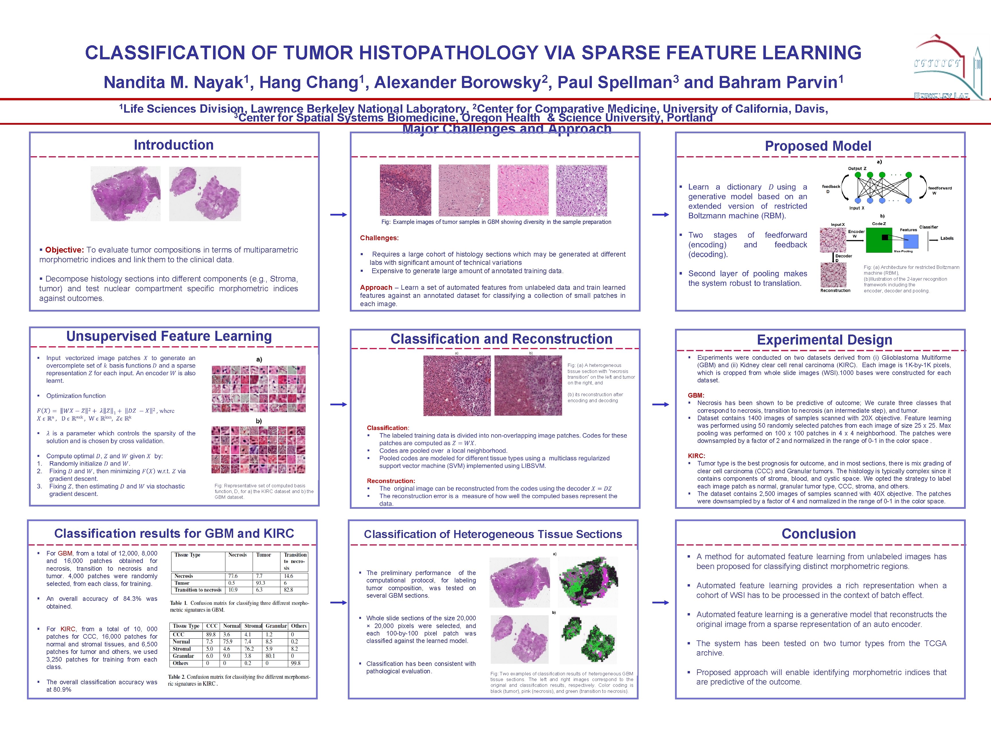
CLASSIFICATION OF TUMOR HISTOPATHOLOGY VIA SPARSE FEATURE LEARNING Nandita M. 1 Life 1 Nayak , Hang 1 Chang , Alexander 2 Borowsky , Paul 3 Spellman and Bahram 1 Parvin 2 Center for Comparative Medicine, University of California, Davis, Sciences Division, Lawrence Berkeley National Laboratory, 3 Center for Spatial Systems Biomedicine, Oregon Health & Science University, Portland Major Challenges and Approach Introduction Proposed Model a) Fig: Example images of tumor samples in GBM showing diversity in the sample preparation Challenges: § Objective: To evaluate tumor compositions in terms of multiparametric morphometric indices and link them to the clinical data. § Decompose histology sections into different components (e. g. , Stroma, tumor) and test nuclear compartment specific morphometric indices against outcomes. Unsupervised Feature Learning Diagram of the proposed method. § Requires a large cohort of histology sections which may be generated at different labs with significant amount of technical variations § Expensive to generate large amount of annotated training data. Fig: (a) Architecture for restricted Boltzmann machine (RBM), (b)Illustration of the 2 -layer recognition framework including the encoder, decoder and pooling. Approach – Learn a set of automated features from unlabeled data and train learned features against an annotated dataset for classifying a collection of small patches in each image. Classification and Reconstruction Experimental Design § Fig: (a) A heterogeneous tissue section with “necrosis transition” on the left and tumor on the right, and (b) its reconstruction after encoding and decoding § § For GBM, from a total of 12, 000, 8, 000 and 16, 000 patches obtained for necrosis, transition to necrosis and tumor. 4, 000 patches were randomly selected, from each class, for training. An overall accuracy of 84. 3% was obtained. For KIRC, from a total of 10, 000 patches for CCC, 16, 000 patches for normal and stromal tissues, and 6, 500 patches for tumor and others, we used 3, 250 patches for training from each class. The overall classification accuracy was at 80. 9% GBM: § Necrosis has been shown to be predictive of outcome; We curate three classes that correspond to necrosis, transition to necrosis (an intermediate step), and tumor. § Dataset contains 1400 images of samples scanned with 20 X objective. Feature learning was performed using 50 randomly selected patches from each image of size 25 x 25. Max pooling was performed on 100 x 100 patches in 4 x 4 neighborhood. The patches were downsampled by a factor of 2 and normalized in the range of 0 -1 in the color space. KIRC: § Tumor type is the best prognosis for outcome, and in most sections, there is mix grading of clear cell carcinoma (CCC) and Granular tumors. The histology is typically complex since it contains components of stroma, blood, and cystic space. We opted the strategy to label each image patch as normal, granular tumor type, CCC, stroma, and others. § The dataset contains 2, 500 images of samples scanned with 40 X objective. The patches were downsampled by a factor of 4 and normalized in the range of 0 -1 in the color space. Fig: Representative set of computed basis function, D, for a) the KIRC dataset and b) the GBM dataset. Classification results for GBM and KIRC Experiments were conducted on two datasets derived from (i) Glioblastoma Multiforme (GBM) and (ii) Kidney clear cell renal carcinoma (KIRC). Each image is 1 K-by-1 K pixels, which is cropped from whole slide images (WSI). 1000 bases were constructed for each dataset. Classification of Heterogeneous Tissue Sections § A method for automated feature learning from unlabeled images has been proposed for classifying distinct morphometric regions. § The preliminary performance of the computational protocol, for labeling tumor composition, was tested on several GBM sections. § Automated feature learning provides a rich representation when a cohort of WSI has to be processed in the context of batch effect. § Automated feature learning is a generative model that reconstructs the original image from a sparse representation of an auto encoder. § Whole slide sections of the size 20, 000 × 20, 000 pixels were selected, and each 100 -by-100 pixel patch was classified against the learned model. § Classification has been consistent with pathological evaluation. Conclusion § The system has been tested on two tumor types from the TCGA archive. Fig: Two examples of classification results of heterogeneous GBM tissue sections. The left and right images correspond to the original and classification results, respectively. Color coding is black (tumor), pink (necrosis), and green (transition to necrosis). § Proposed approach will enable identifying morphometric indices that are predictive of the outcome.