Classification of parallel computers Limitations of parallel processing

Classification of parallel computers Limitations of parallel processing

Classification of parallel computers n 1966 M. J. Flynn has made an informal classification of computer parallelism based on the number of simultaneous instruction and data streams, which can be distinguished during operation of a computer system

Classification of parallel computers SISD IS CU PU – Processing Unit CU – Control Unit MM – Memory Module n PU DS MM IS – Instruction Stream DS – Data Stream Single Instruction Stream Single Data Stream n n Conventional architectures (von Neumann’s) Vector computers?

Classification of parallel computers SIMD PE 1 IS CU PE 2 PEn n DS 1 DS 2 DSn MM 1 MM 2 MMm Single Instruction Stream Multiple Data Streams n n Vector computers? Array computers

Classification of parallel computers MISD IS 1 IS 2 DS. CU 1 PU 1 MM 1 CU 2 PU 2 MM 2 CUn PUn ISn n MMm Multiple Instruction Streams Single Data Stream n Nonexistent, systolic array, pipelining?

Classification of parallel computers MIMD IS 1 IS 2 ISn n CU 1 CU 2 CUn PE 1 PE 2 PEn DS 1 DS 2 DSn MM 1 MM 2 MMm Multiple Instruction Streams Multiple Data Streams n n Multiprocessor systems Multicomputer systems

Classification of parallel computers M. J. Flynn n Advantages of classification n n Simplicity Disadvantages n n n Does not include all solutions and classes MISD is an empty layer MIMD is overloaded layer

Classification of parallel computers according to sources of parallelism n Data-level parallelism n n Instruction-level parallelism (low-level parallelism) n n The same operation performed on multiple data units Instruction Pipelining Multiple Processor Functional Units Data flow analysis / out-of-order execution / branch prediction Process/Thread-level parallelism (high-level parallelism)

Time Classification of parallel computers according to sources of parallelism Instruction-Level Parallelism (ILP) Time Data-Level Parallelism (DLP) Thread-Level Parallelism (TLP)

First mechanisms of parallel processing n Evolution of I/O functions n n Development of memory n n n Interrupts DMA I/O processors Virtual memory Cache memory Multiplied ALUs (IBM 360, CDC 6600)

First mechanisms of parallel processing n Pipelining n n Pipelined control unit (Instruction Pipelining) Pipelined arithmetic-logic unit (Arithmetic pipelining)

Limitations of parallel processing n How much faster is my program going to be run on a parallel computer than on a machine without any mechanisms of parallel processing (uniprocessor)?

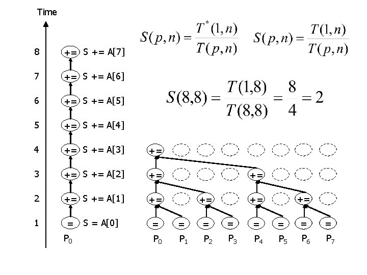
Time and Processor Complexity n Given an algorithm and an input data of a given size n n Time complexity T(n) is a number of time steps needed to execute the algorithm for the given input of size n Processor complexity P(n) is a number of processors used in the execution of the algorithm for the given input of size n T(p, n) is a number of time steps needed to execute the algorithm on p processors for the given input of size n

Speedup n Speedup S(p, n) gives the factor of acceleration going from a sequential execution of an algorithm on one processor to the parallel execution of the parallel algorithm on p processors

Speedup n n T*(1, n) is the execution time for the best known sequential algorithm Typically 1<= S(p, n) <= p n n S(p, n) = p – ideal speedup S(p, n) > p – superlinear speedup

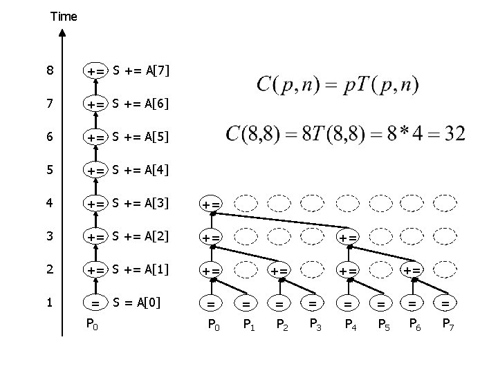
Cost n n Cost is execution times number of processors A cost-optimal algorithm is an algorithm for which the cost to solve a problem on parallel system is proportional to the cost on a single processor

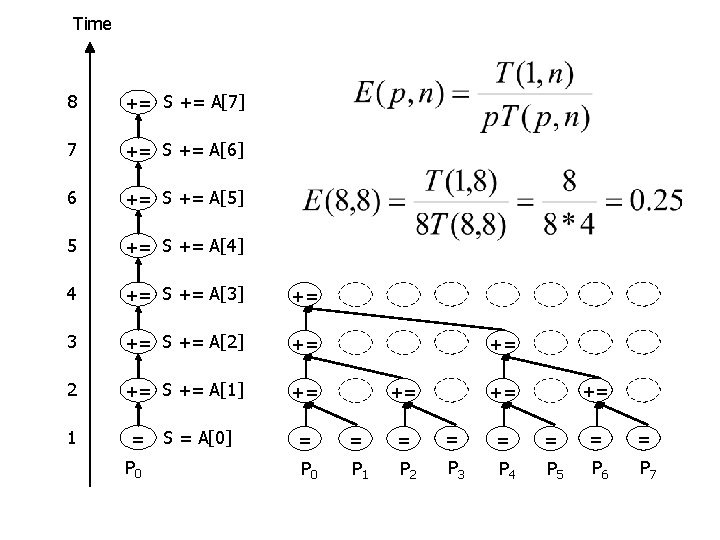
Efficiency n n Efficiency relates the speedup to a number of processors Efficiency represents fraction of time for which a processor does a useful work

Amdahl’s Law n Assuming the constant size of a problem, what is the maximum speedup that can be obtained with the use of parallel processing?

Amdahl’s Law 1 p=1 f 1 -f Sequential part Perfectly parallelizable part p=2 f p=4 f (1 -f) / 2 (1 -f) / 4

Amdahl’s Law

Gustafson’s Law n n Is the reduced execution time obtained thanks to parallel processing always of the highest priority? What about the increased amount of work that can be performed thanks to application of parallel processing within the same period of time?

Gustafson’s Law 1 p=1 f 1 -f Sequential part Perfectly parallelizable part p=2 f 1 -f p=4 f 1 -f

Gustafson’s Law

Grain of parallelism n n Fine grain of parallelism type of problems Coarse grain of parallelism type of problems

Loosely & Tightly Coupled Design Approach n n Loosely & tightly coupled design approach represents the degree of internal coupling between components of the computer system Mentioned degree of coupling corresponds to the overhead associated with the communication as well as the potential to upscale a given design