Classification Methods Definition of Classification Classification or more

Classification Methods

Definition of Classification ß Classification, or more specifically, statistical classification, is a problem of identifying to which of a set of categories (sub-populations) a new observation belongs, on the basis of a training set of data containing observations (or instances) whose category membership is known.

The Importance of Classification ß ß The most straight-forward way for a computer program to understand human intelligence. The fundamental way for computer intelligence to understand this world by true (1) or false (0).

Types of Classification Methods ß ß ß Unsupervised learning: grouping a set of objects in such a way that objects in the same group (called a cluster) are more similar (in some sense or another) to each other than to those in other groups (clusters). Supervised learning: (Next Slide) Hybrid learning method.

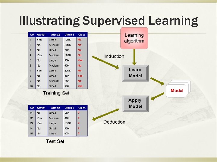
Supervised Learning: Definition ß Given a collection of records (training set ) Þ ß ß Each record contains a set of attributes, one of the attributes is the class. Find a model for class attribute as a function of the values of other attributes. Goal: previously unseen records should be assigned a class as accurately as possible. Þ A test set is used to determine the accuracy of the model. Usually, the given data set is divided into training and test sets, with training set used to build the model and test set used to validate it.

Illustrating Supervised Learning

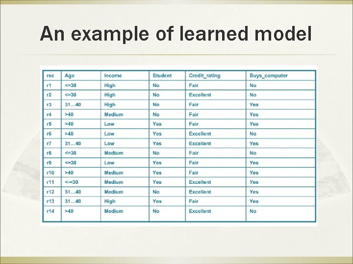
An example of learned model

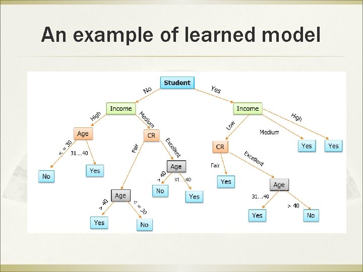
An example of learned model

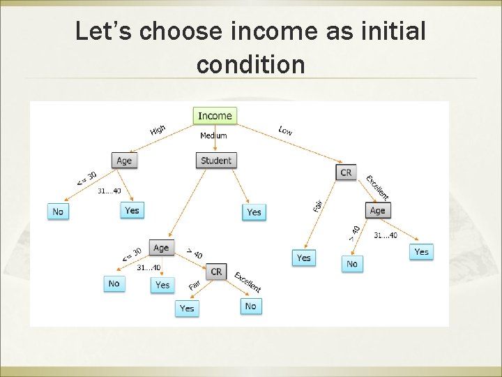
Let’s choose income as initial condition

An example application ß ß An emergency room in a hospital measures 17 variables (e. g. , blood pressure, age, etc) of newly admitted patients. A decision is needed: whether to put a new patient in an intensive-care unit. Due to the high cost of ICU, those patients who may survive less than a month are given higher priority. Problem: to predict high-risk patients and discriminate them from low-risk patients. 10

Another application ß A credit card company receives thousands of applications for new cards. Each application contains information about an applicant, Þ Þ Þ ß age Marital status annual salary outstanding debts credit rating etc. Problem: to decide whether an application should approved, or to classify applications into two categories, approved and not approved. 11

Machine learning and our focus ß ß ß Like human learning from past experiences. A computer does not have “experiences”. A computer system learns from data, which represent some “past experiences” of an application domain. Our focus: learn a target function that can be used to predict the values of a discrete class attribute, e. g. , approve or not-approved, and high-risk or low risk. The task is commonly called: Supervised learning, classification, or inductive learning. 12

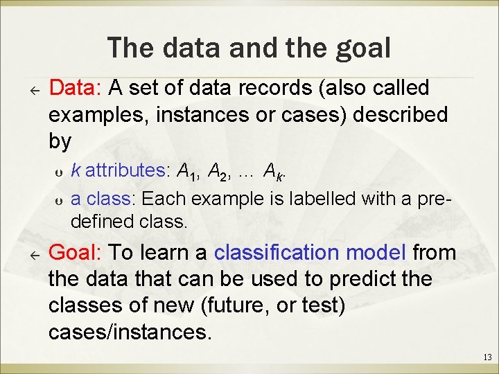
The data and the goal ß Data: A set of data records (also called examples, instances or cases) described by Þ Þ ß k attributes: A 1, A 2, … Ak. a class: Each example is labelled with a predefined class. Goal: To learn a classification model from the data that can be used to predict the classes of new (future, or test) cases/instances. 13

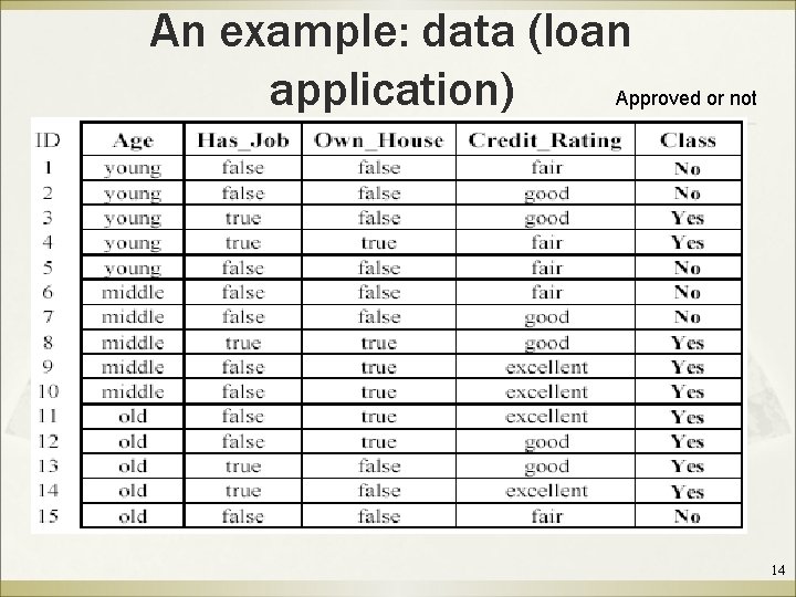
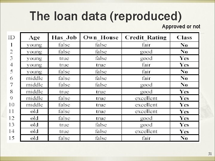
An example: data (loan application) Approved or not 14

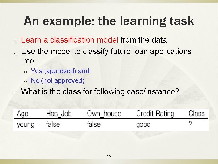
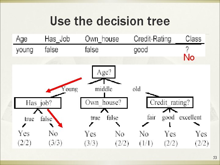
An example: the learning task ß ß Learn a classification model from the data Use the model to classify future loan applications into Þ Þ ß Yes (approved) and No (not approved) What is the class for following case/instance? 15

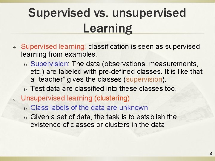
Supervised vs. unsupervised Learning ß ß Supervised learning: classification is seen as supervised learning from examples. Þ Supervision: The data (observations, measurements, etc. ) are labeled with pre-defined classes. It is like that a “teacher” gives the classes (supervision). Þ Test data are classified into these classes too. Unsupervised learning (clustering) Þ Class labels of the data are unknown Þ Given a set of data, the task is to establish the existence of classes or clusters in the data 16

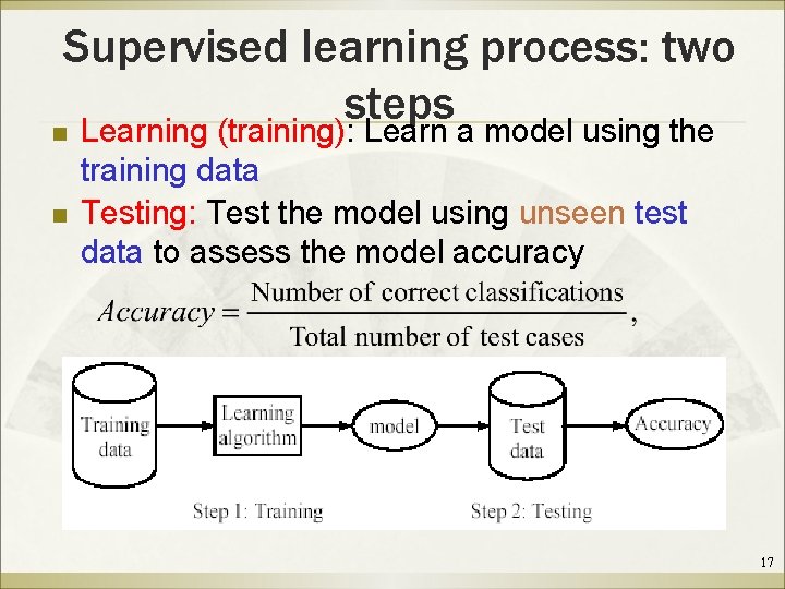
Supervised learning process: two steps n Learning (training): Learn a model using the n training data Testing: Test the model using unseen test data to assess the model accuracy 17

What do we mean by learning? ß Given Þ Þ Þ ß a data set D, a task T, and a performance measure M, a computer system is said to learn from D to perform the task T if after learning the system’s performance on T improves as measured by M. In other words, the learned model helps the system to perform T better as compared to no learning. 18

An example ß ß ß Data: Loan application data Task: Predict whether a loan should be approved or not. Performance measure: accuracy. No learning: classify all future applications (test data) to the majority class (i. e. , Yes): Accuracy = 9/15 = 60%. ß We can do better than 60% with learning. 19

Fundamental assumption of learning Assumption: The distribution of training examples is identical to the distribution of test examples (including future unseen examples). ß ß ß In practice, this assumption is often violated to certain degree. Strong violations will clearly result in poor classification accuracy. To achieve good accuracy on the test data, training examples must be sufficiently representative of the test data. 20

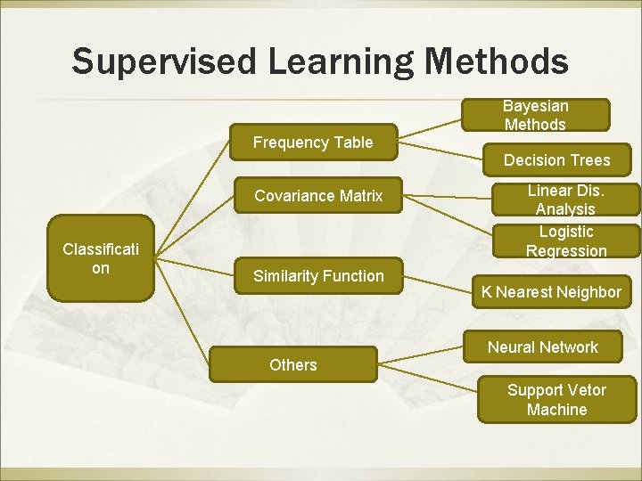
Supervised Learning Methods Frequency Table Covariance Matrix Classificati on Similarity Function Others Bayesian Methods Decision Trees Linear Dis. Analysis Logistic Regression K Nearest Neighbor Neural Network Support Vetor Machine

Bayesian Classification Methods ß ß The Bayesian Classification represents a supervised learning method. Assumes an underlying probabilistic model and it allows us to capture uncertainty about the model in a principled way by determining probabilities of the outcomes. It can solve diagnostic and predictive problems.

Bayesian Classification Methods ß ß This Classification is named after Thomas Bayes ( 1702 -1761), who proposed the Bayes classification methods. Bayesian classification provides practical learning algorithms and prior knowledge and observed data can be combined. Bayesian Classification provides a useful perspective for understanding and evaluating many learning algorithms. It calculates explicit probabilities for hypothesis and it is robust to noise in input data

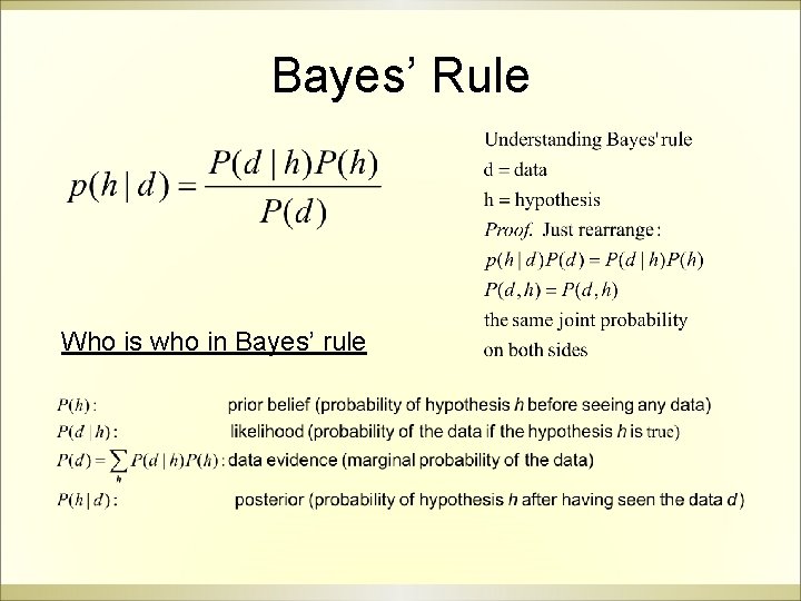
Bayes’ Rule Who is who in Bayes’ rule

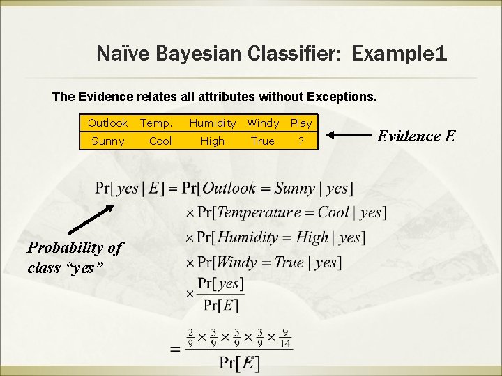
Naïve Bayesian Classifier: Example 1 The Evidence relates all attributes without Exceptions. Outlook Sunny Temp. Cool Humidity Windy High True Probability of class “yes” 25 Play ? Evidence E

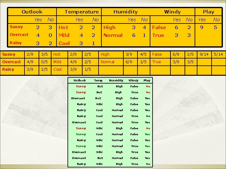
Outlook Temperature Yes Humidity No Yes Windy Yes No No Sunny 2 3 Hot 2 2 High 3 4 Overcast 4 0 Mild 4 2 Normal 6 1 Rainy 3 2 Cool 3 1 Play Yes No False 6 2 9 5 True 3 3 9/14 5/14 Sunny 2/9 3/5 Hot 2/9 2/5 High 3/9 4/5 False 6/9 2/5 Overcast 4/9 0/5 Mild 4/9 2/5 Normal 6/9 1/5 True 3/9 3/5 Rainy 3/9 2/5 Cool 3/9 1/5 Outlook Temp Humidity Windy Play Sunny Hot High False No True No High False Yes Sunny Overcast Hot High Hot Rainy Mild High False Yes Rainy Cool Normal True No Overcast Cool Normal True Yes Sunny Mild High False No Sunny Cool Normal False Yes Rainy Mild Normal False Yes Sunny Mild Normal True Yes Overcast Mild High True Yes Overcast Hot Normal False Yes Rainy Mild High True No 26

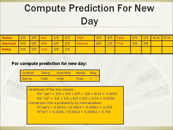
Compute Prediction For New Day Sunny 2/9 3/5 Hot 2/9 2/5 High 3/9 4/5 False 6/9 2/5 Overcast 4/9 0/5 Mild 4/9 2/5 Normal 6/9 1/5 True 3/9 3/5 Rainy 3/9 2/5 Cool 3/9 1/5 For compute prediction for new day: Outlook Temp. Humidity Windy Play Sunny Cool High True ? Likelihood of the two classes For “yes” = 2/9 3/9 9/14 = 0. 0053 For “no” = 3/5 1/5 4/5 3/5 5/14 = 0. 0206 Conversion into a probability by normalization: P(“yes”) = 0. 0053 / (0. 0053 + 0. 0206) = 0. 205 P(“no”) = 0. 0206 / (0. 0053 + 0. 0206) = 0. 795 27 9/14 5/14

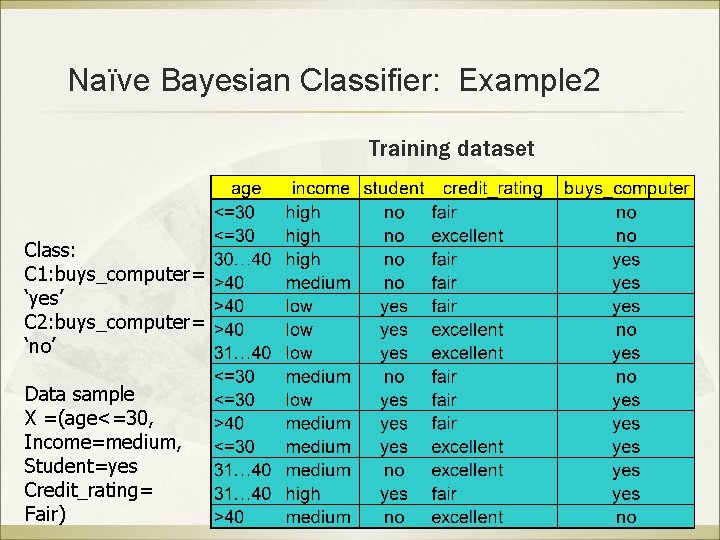
Naïve Bayesian Classifier: Example 2 Training dataset Class: C 1: buys_computer= ‘yes’ C 2: buys_computer= ‘no’ Data sample X =(age<=30, Income=medium, Student=yes Credit_rating= Fair) 28

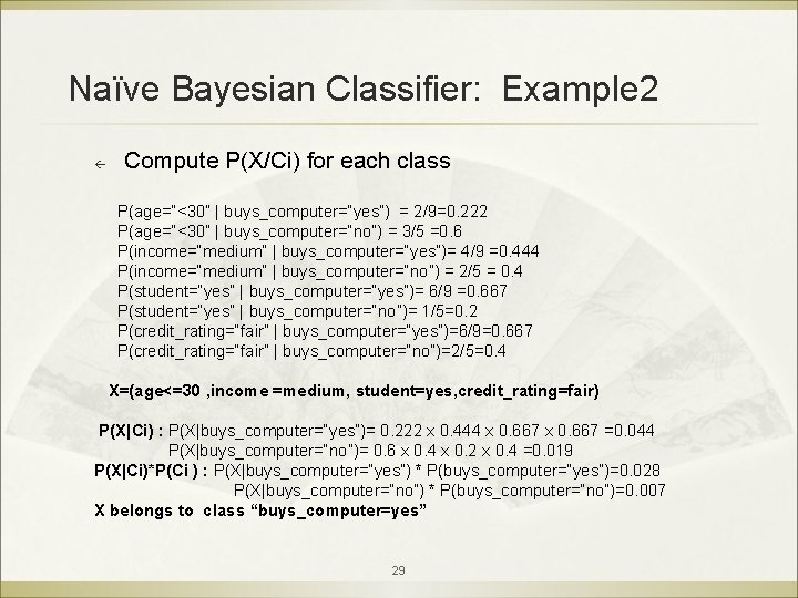
Naïve Bayesian Classifier: Example 2 ß Compute P(X/Ci) for each class P(age=“<30” | buys_computer=“yes”) = 2/9=0. 222 P(age=“<30” | buys_computer=“no”) = 3/5 =0. 6 P(income=“medium” | buys_computer=“yes”)= 4/9 =0. 444 P(income=“medium” | buys_computer=“no”) = 2/5 = 0. 4 P(student=“yes” | buys_computer=“yes”)= 6/9 =0. 667 P(student=“yes” | buys_computer=“no”)= 1/5=0. 2 P(credit_rating=“fair” | buys_computer=“yes”)=6/9=0. 667 P(credit_rating=“fair” | buys_computer=“no”)=2/5=0. 4 X=(age<=30 , income =medium, student=yes, credit_rating=fair) P(X|Ci) : P(X|buys_computer=“yes”)= 0. 222 x 0. 444 x 0. 667 =0. 044 P(X|buys_computer=“no”)= 0. 6 x 0. 4 x 0. 2 x 0. 4 =0. 019 P(X|Ci)*P(Ci ) : P(X|buys_computer=“yes”) * P(buys_computer=“yes”)=0. 028 P(X|buys_computer=“no”) * P(buys_computer=“no”)=0. 007 X belongs to class “buys_computer=yes” 29

Naïve Bayesian Classifier: Advantages and Disadvantages ß Advantages : Þ Þ ß Easy to implement. Good results obtained in most of the cases. Disadvantages Assumption: class conditional independence , therefore loss of accuracy Þ Practically, dependencies exist among variables Þ E. g. , hospital patients’profile: age, family history etc Symptoms: fever, cough etc. , Disease: lung cancer, diabetes etc Þ Dependencies among these cannot be modeled by Naïve Bayesian Classifier. Þ ß How to deal with these dependencies? Þ Bayesian Belief Networks. 30

Supervised Learning Methods Frequency Table Covariance Matrix Classificati on Similarity Function Others Bayesian Methods Decision Trees Linear Dis. Analysis Logistic Regression K Nearest Neighbor Neural Network Support Vetor Machine

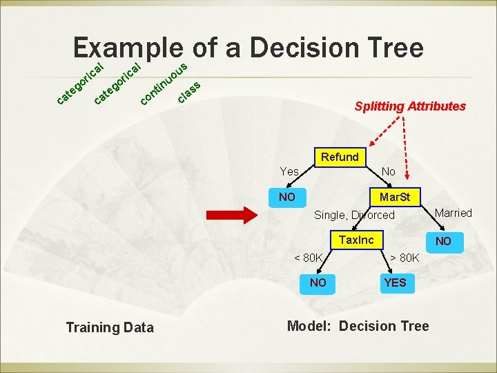
Example of a Decision Tree al ric c at o eg c at al o eg ric in nt co u s u o ss a cl Splitting Attributes Refund Yes No NO Mar. St Single, Divorced Tax. Inc < 80 K NO Training Data Married NO > 80 K YES Model: Decision Tree

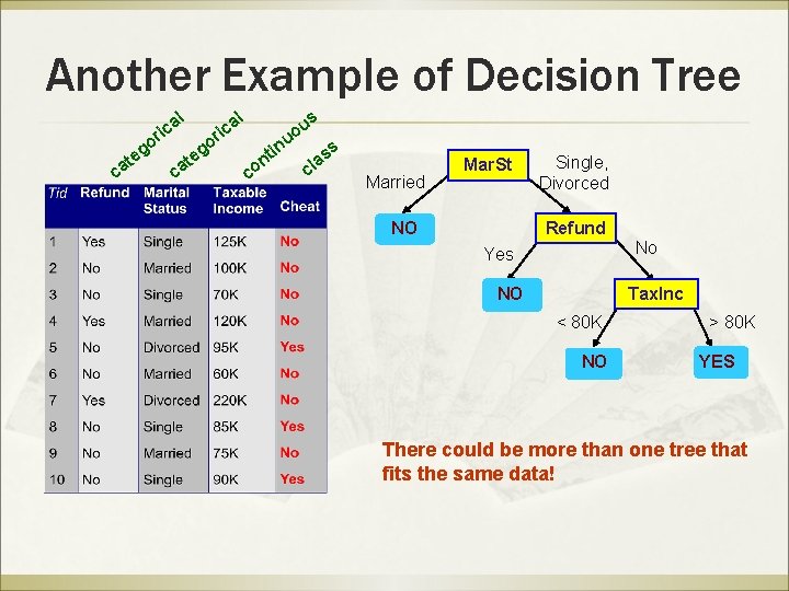
Another Example of Decision Tree l ca g te l a ric o o ca g te s a ric u uo co in t n ss a cl Married Mar. St NO Single, Divorced Refund No Yes NO Tax. Inc < 80 K NO > 80 K YES There could be more than one tree that fits the same data!

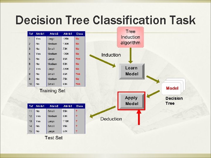
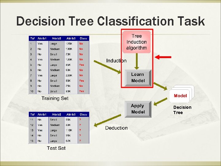
Decision Tree Classification Task Decision Tree

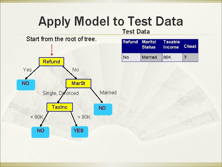
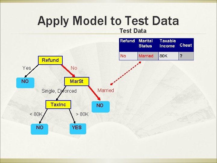
Apply Model to Test Data Start from the root of tree. Refund Yes No NO Mar. St Single, Divorced Tax. Inc < 80 K NO Married NO > 80 K YES

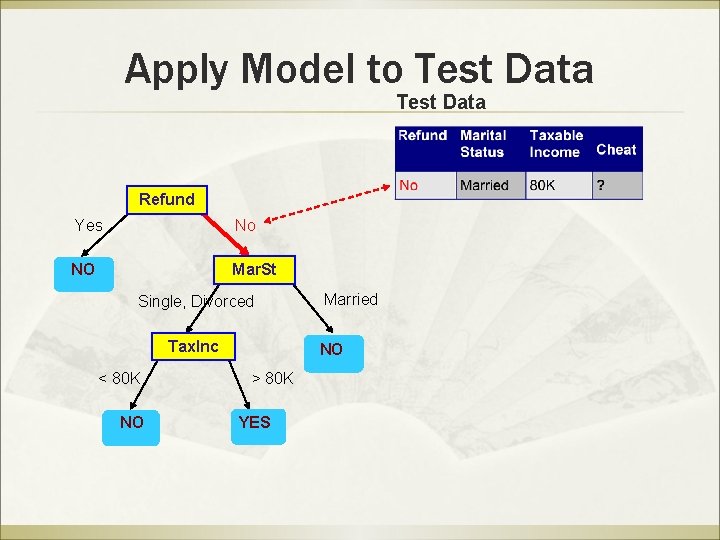
Apply Model to Test Data Refund Yes No NO Mar. St Single, Divorced Tax. Inc < 80 K NO Married NO > 80 K YES

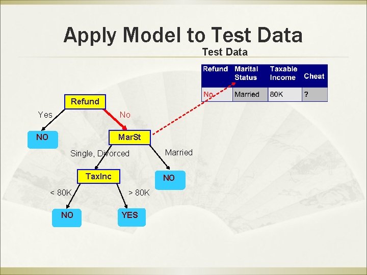
Apply Model to Test Data Refund Yes No NO Mar. St Single, Divorced Tax. Inc < 80 K NO Married NO > 80 K YES

Apply Model to Test Data Refund Yes No NO Mar. St Single, Divorced Tax. Inc < 80 K NO Married NO > 80 K YES

Apply Model to Test Data Refund Yes No NO Mar. St Single, Divorced Tax. Inc < 80 K NO Married NO > 80 K YES

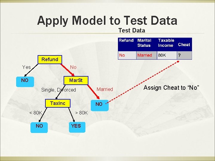
Apply Model to Test Data Refund Yes No NO Mar. St Single, Divorced Tax. Inc < 80 K NO Married NO > 80 K YES Assign Cheat to “No”

Decision Tree Classification Task Decision Tree

Decision Tree Induction ß Many Algorithms: Þ Þ Hunt’s Algorithm (one of the earliest) CART ID 3, C 4. 5 SLIQ, SPRINT

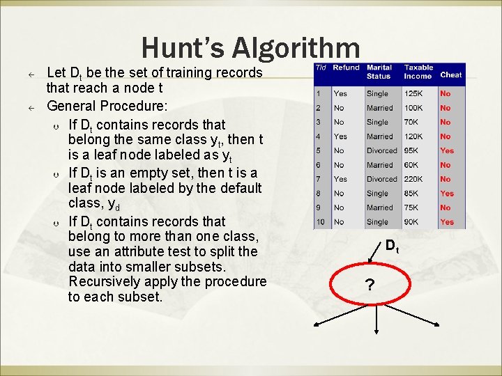
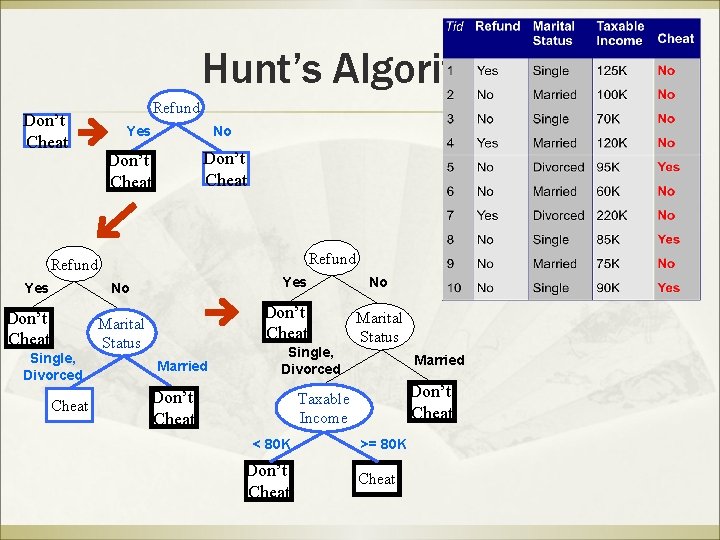
Hunt’s Algorithm ß ß Let Dt be the set of training records that reach a node t General Procedure: Þ If Dt contains records that belong the same class yt, then t is a leaf node labeled as yt Þ If Dt is an empty set, then t is a leaf node labeled by the default class, yd Þ If Dt contains records that belong to more than one class, use an attribute test to split the data into smaller subsets. Recursively apply the procedure to each subset. Dt ?

Hunt’s Algorithm Don’t Cheat Refund Yes No Don’t Cheat Single, Divorced Cheat Don’t Cheat Marital Status Married Single, Divorced Don’t Cheat No Marital Status Married Don’t Cheat Taxable Income < 80 K Don’t Cheat >= 80 K Cheat

Tree Induction ß Greedy strategy. Þ ß Split the records based on an attribute test that optimizes certain criterion. Issues Þ Determine how to split the records How to specify the attribute test condition? How to determine the best split? Þ Determine when to stop splitting

How to Specify Test Condition? ß Depends on attribute types Þ Þ Þ ß Nominal Ordinal Continuous Depends on number of ways to split Þ Þ 2 -way split Multi-way split

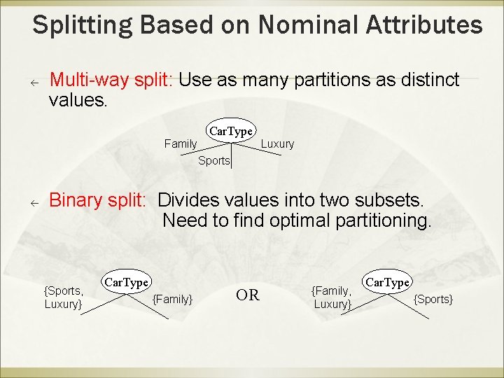
Splitting Based on Nominal Attributes ß Multi-way split: Use as many partitions as distinct values. Car. Type Family Luxury Sports ß Binary split: Divides values into two subsets. Need to find optimal partitioning. {Sports, Luxury} Car. Type {Family} OR {Family, Luxury} Car. Type {Sports}

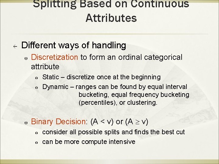
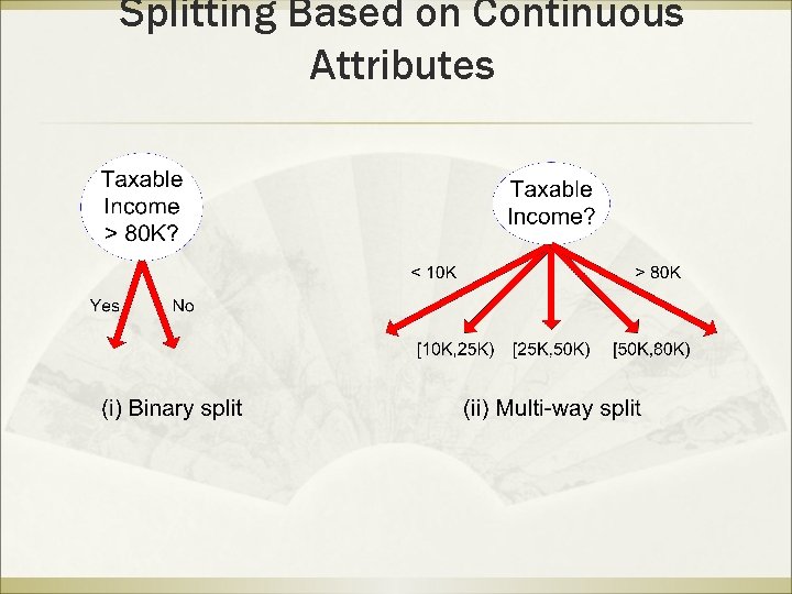
Splitting Based on Continuous Attributes ß Different ways of handling Þ Discretization to form an ordinal categorical attribute Þ Static – discretize once at the beginning Dynamic – ranges can be found by equal interval bucketing, equal frequency bucketing (percentiles), or clustering. Binary Decision: (A < v) or (A v) consider all possible splits and finds the best cut can be more compute intensive

Splitting Based on Continuous Attributes

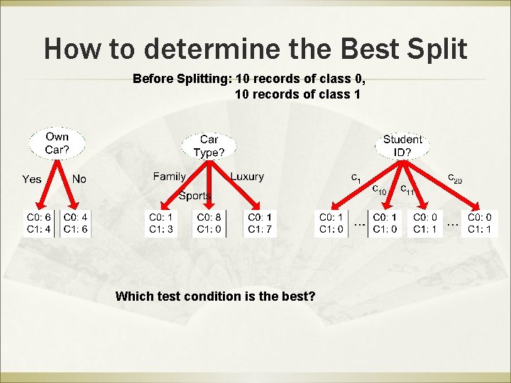
How to determine the Best Split Before Splitting: 10 records of class 0, 10 records of class 1 Which test condition is the best?

The loan data (reproduced) Approved or not 51

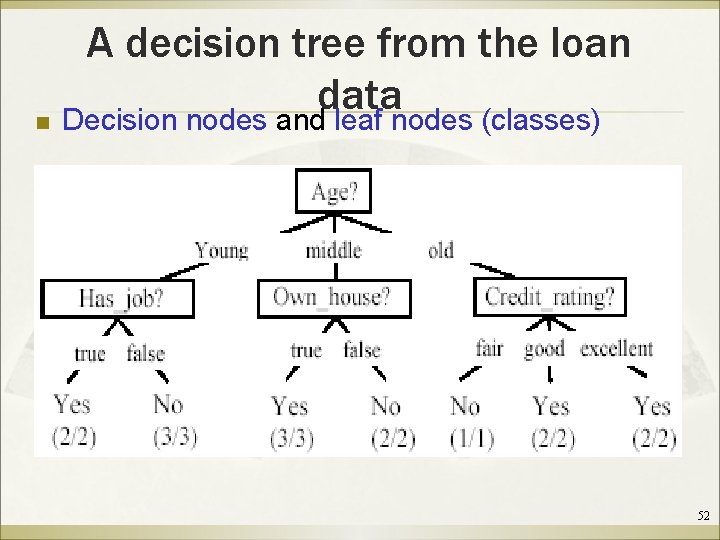
A decision tree from the loan data n Decision nodes and leaf nodes (classes) 52

Use the decision tree No 53

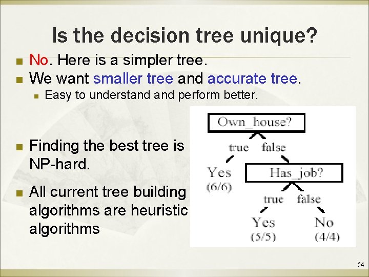
Is the decision tree unique? n n No. Here is a simpler tree. We want smaller tree and accurate tree. n Easy to understand perform better. n Finding the best tree is NP-hard. n All current tree building algorithms are heuristic algorithms 54

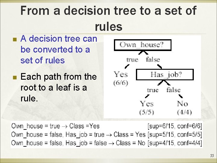
From a decision tree to a set of rules n A decision tree can be converted to a set of rules n Each path from the root to a leaf is a rule. 55

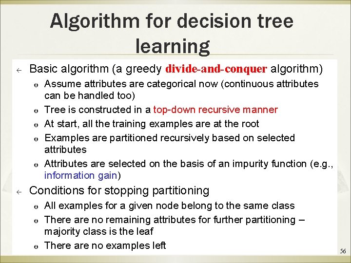
Algorithm for decision tree learning ß Basic algorithm (a greedy divide-and-conquer algorithm) Þ Þ Þ ß Assume attributes are categorical now (continuous attributes can be handled too) Tree is constructed in a top-down recursive manner At start, all the training examples are at the root Examples are partitioned recursively based on selected attributes Attributes are selected on the basis of an impurity function (e. g. , information gain) Conditions for stopping partitioning Þ Þ Þ All examples for a given node belong to the same class There are no remaining attributes for further partitioning – majority class is the leaf There are no examples left 56

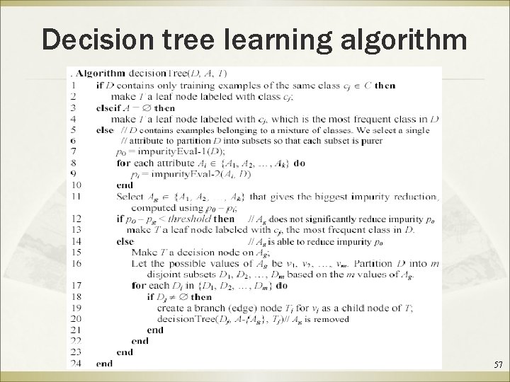
Decision tree learning algorithm 57

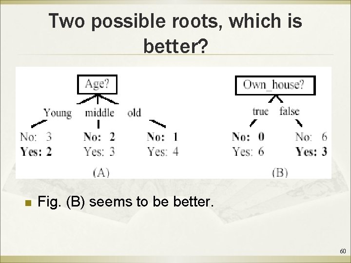
Choose an attribute to partition data ß ß The key to building a decision tree - which attribute to choose in order to branch. The objective is to reduce impurity or uncertainty in data as much as possible. Þ ß A subset of data is pure if all instances belong to the same class. The heuristic in C 4. 5 is to choose the attribute with the maximum Information Gain or Gain Ratio based on information theory. 58

The loan data (reproduced) Approved or not 59

Two possible roots, which is better? n Fig. (B) seems to be better. 60

Information theory ß ß Information theory provides a mathematical basis for measuring the information content. To understand the notion of information, think about it as providing the answer to a question, for example, whether a coin will come up heads. Þ Þ If one already has a good guess about the answer, then the actual answer is less informative. If one already knows that the coin is rigged so that it will come with heads with probability 0. 99, then a message (advanced information) about the actual outcome of a flip is worth less than it would be for a honest coin (50 -50). 61

Information theory (cont …) ß ß ß For a fair (honest) coin, you have no information, and you are willing to pay more (say in terms of $) for advanced information - less you know, the more valuable the information. Information theory uses this same intuition, but instead of measuring the value for information in dollars, it measures information contents in bits. One bit of information is enough to answer a yes/no question about which one has no idea, such as the flip of a fair coin 62

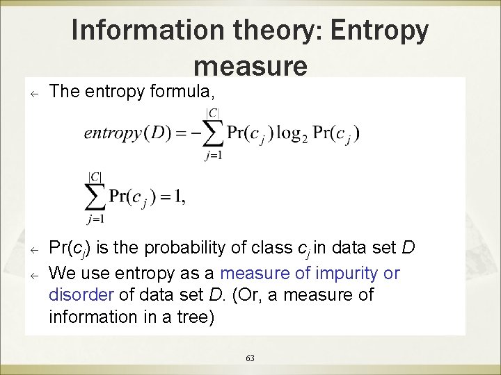
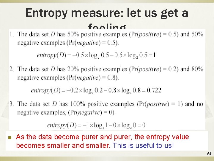
Information theory: Entropy measure ß ß ß The entropy formula, Pr(cj) is the probability of class cj in data set D We use entropy as a measure of impurity or disorder of data set D. (Or, a measure of information in a tree) 63

Entropy measure: let us get a feeling n As the data become purer and purer, the entropy value becomes smaller and smaller. This is useful to us! 64

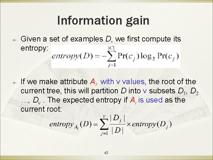
Information gain ß ß Given a set of examples D, we first compute its entropy: If we make attribute Ai, with v values, the root of the current tree, this will partition D into v subsets D 1, D 2 …, Dv. The expected entropy if Ai is used as the current root: 65

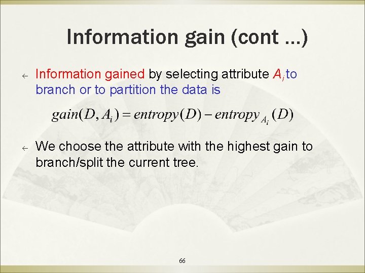
Information gain (cont …) ß ß Information gained by selecting attribute Ai to branch or to partition the data is We choose the attribute with the highest gain to branch/split the current tree. 66

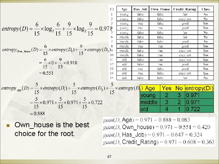
n Own_house is the best choice for the root. 67

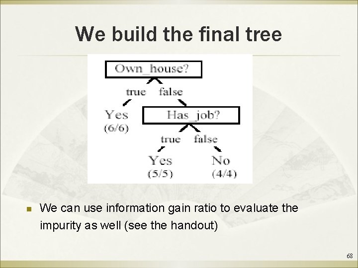
We build the final tree n We can use information gain ratio to evaluate the impurity as well (see the handout) 68

QUIZ ß ß 1. Naive Bayes Method 2. Decision Tree Method

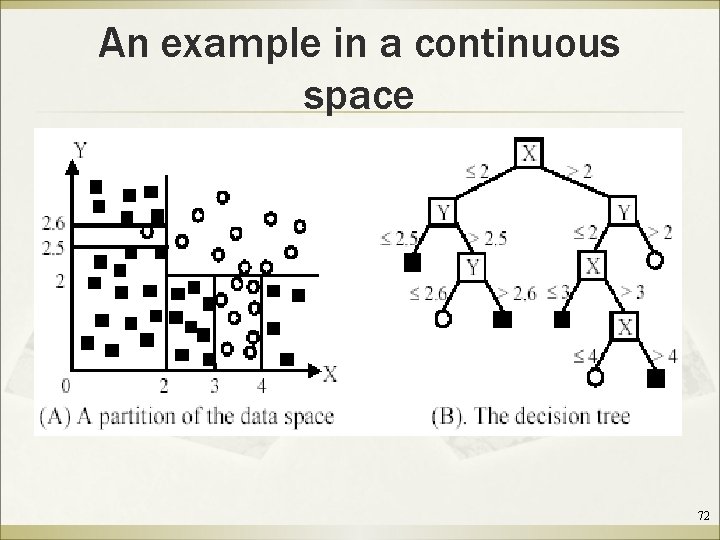
Handling continuous attributes ß ß Handle continuous attribute by splitting into two intervals (can be more) at each node. How to find the best threshold to divide? Þ Use information gain or gain ratio again Þ Sort all the values of an continuous attribute in increasing order {v 1, v 2, …, vr}, Þ One possible threshold between two adjacent values vi and vi+1. Try all possible thresholds and find the one that maximizes the gain (or gain ratio). 71

An example in a continuous space 72

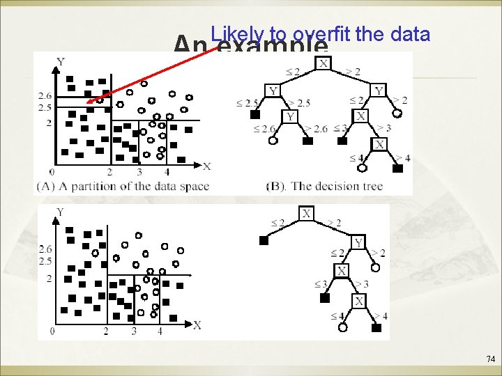
Avoid overfitting in classification ß ß Overfitting: A tree may overfit the training data Þ Good accuracy on training data but poor on test data Þ Symptoms: tree too deep and too many branches, some may reflect anomalies due to noise or outliers Two approaches to avoid overfitting Þ Pre-pruning: Halt tree construction early Difficult to decide because we do not know what may happen subsequently if we keep growing the tree. Þ Post-pruning: Remove branches or sub-trees from a “fully grown” tree. This method is commonly used. C 4. 5 uses a statistical method to estimates the errors at each node for pruning. A validation set may be used for pruning as well. 73

Likely to overfit the data An example 74

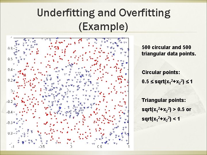
Underfitting and Overfitting (Example) 500 circular and 500 triangular data points. Circular points: 0. 5 sqrt(x 12+x 22) 1 Triangular points: sqrt(x 12+x 22) > 0. 5 or sqrt(x 12+x 22) < 1

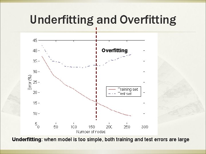
Underfitting and Overfitting Underfitting: when model is too simple, both training and test errors are large

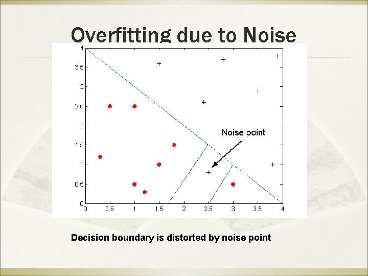
Overfitting due to Noise Decision boundary is distorted by noise point

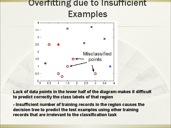
Overfitting due to Insufficient Examples Lack of data points in the lower half of the diagram makes it difficult to predict correctly the class labels of that region - Insufficient number of training records in the region causes the decision tree to predict the test examples using other training records that are irrelevant to the classification task

Notes on Overfitting ß ß ß Overfitting results in decision trees that are more complex than necessary Training error no longer provides a good estimate of how well the tree will perform on previously unseen records Need new ways for estimating errors

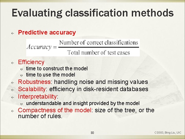
Evaluating classification methods ß Predictive accuracy ß Efficiency Þ Þ ß ß ß Robustness: handling noise and missing values Scalability: efficiency in disk-resident databases Interpretability: Þ ß time to construct the model time to use the model understandable and insight provided by the model Compactness of the model: size of the tree, or the number of rules. 80 CS 583, Bing Liu, UIC

Evaluation methods ß Holdout set: The available data set D is divided into two disjoint subsets, Þ Þ ß Important: training set should not be used in testing and the test set should not be used in learning. Þ ß ß the training set Dtrain (for learning a model) the test set Dtest (for testing the model) Unseen test set provides a unbiased estimate of accuracy. The test set is also called the holdout set. (the examples in the original data set D are all labeled with classes. ) This method is mainly used when the data set D is large. CS 583, Bing Liu, UIC 81

Evaluation methods (cont…) ß ß ß n-fold cross-validation: The available data is partitioned into n equal-size disjoint subsets. Use each subset as the test set and combine the rest n-1 subsets as the training set to learn a classifier. The procedure is run n times, which give n accuracies. The final estimated accuracy of learning is the average of the n accuracies. 10 -fold and 5 -fold cross-validations are commonly used. This method is used when the available data is not large. CS 583, Bing Liu, UIC 82

Evaluation methods (cont…) ß ß Leave-one-out cross-validation: This method is used when the data set is very small. It is a special case of cross-validation Each fold of the cross validation has only a single test example and all the rest of the data is used in training. If the original data has m examples, this is m-fold cross-validation CS 583, Bing Liu, UIC 83

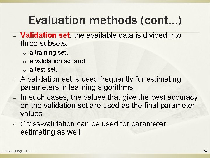
Evaluation methods (cont…) ß Validation set: the available data is divided into three subsets, Þ Þ Þ ß ß ß a training set, a validation set and a test set. A validation set is used frequently for estimating parameters in learning algorithms. In such cases, the values that give the best accuracy on the validation set are used as the final parameter values. Cross-validation can be used for parameter estimating as well. CS 583, Bing Liu, UIC 84

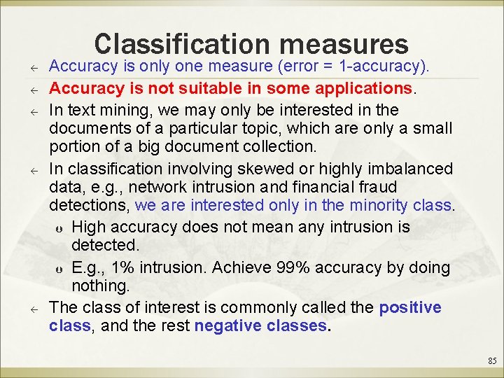
Classification measures ß ß ß Accuracy is only one measure (error = 1 -accuracy). Accuracy is not suitable in some applications. In text mining, we may only be interested in the documents of a particular topic, which are only a small portion of a big document collection. In classification involving skewed or highly imbalanced data, e. g. , network intrusion and financial fraud detections, we are interested only in the minority class. Þ High accuracy does not mean any intrusion is detected. Þ E. g. , 1% intrusion. Achieve 99% accuracy by doing nothing. The class of interest is commonly called the positive class, and the rest negative classes. 85

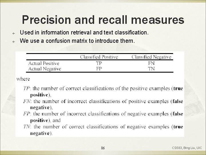
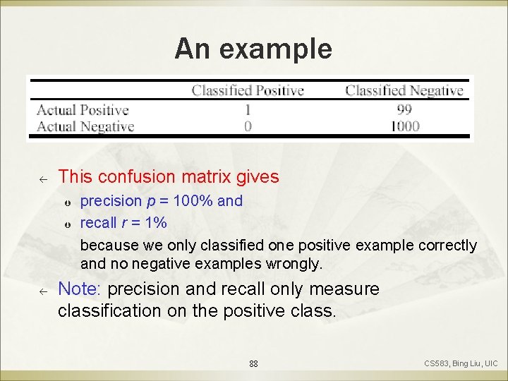
Precision and recall measures ß ß Used in information retrieval and text classification. We use a confusion matrix to introduce them. 86 CS 583, Bing Liu, UIC

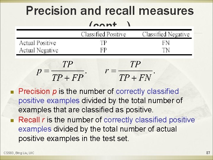
Precision and recall measures (cont…) n n Precision p is the number of correctly classified positive examples divided by the total number of examples that are classified as positive. Recall r is the number of correctly classified positive examples divided by the total number of actual positive examples in the test set. CS 583, Bing Liu, UIC 87

An example ß This confusion matrix gives Þ Þ ß precision p = 100% and recall r = 1% because we only classified one positive example correctly and no negative examples wrongly. Note: precision and recall only measure classification on the positive class. 88 CS 583, Bing Liu, UIC

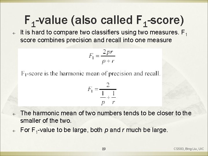
F 1 -value (also called F 1 -score) ß ß ß It is hard to compare two classifiers using two measures. F 1 score combines precision and recall into one measure The harmonic mean of two numbers tends to be closer to the smaller of the two. For F 1 -value to be large, both p and r much be large. 89 CS 583, Bing Liu, UIC

Supervised Learning Methods Frequency Table Covariance Matrix Classificati on Similarity Function Others Bayesian Methods Decision Trees Linear Dis. Analysis Logistic Regression K Nearest Neighbor Neural Network Support Vector Machine

K-Nearest-Neighbors Algorithm and Its Application

K-Nearest-Neighbors Algorithm ß ß K nearest neighbors (KNN) is a simple algorithm that stores all available cases and classifies new cases based on a similarity measure (distance function) KNN has been used in statistical estimation and pattern recognition since 1970’s.

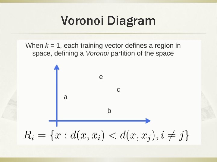
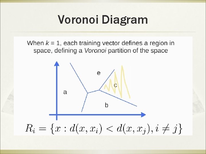
K-Nearest-Neighbors Algorithm ß ß A case is classified by a majority voting of its neighbors, with the case being assigned to the class most common among its K nearest neighbors measured by a distance function. If K=1, then the case is simply assigned to the class of its nearest neighbor

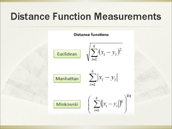
Distance Function Measurements

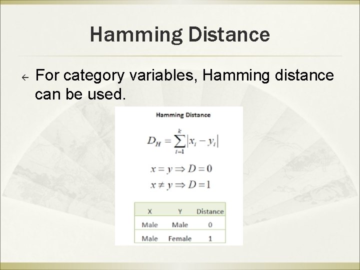
Hamming Distance ß For category variables, Hamming distance can be used.

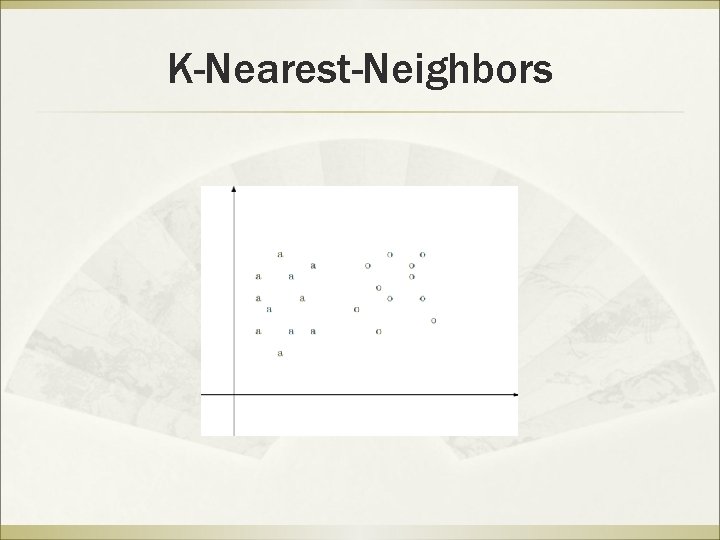
K-Nearest-Neighbors

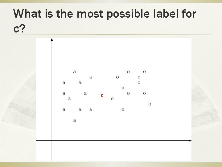
What is the most possible label for c? c

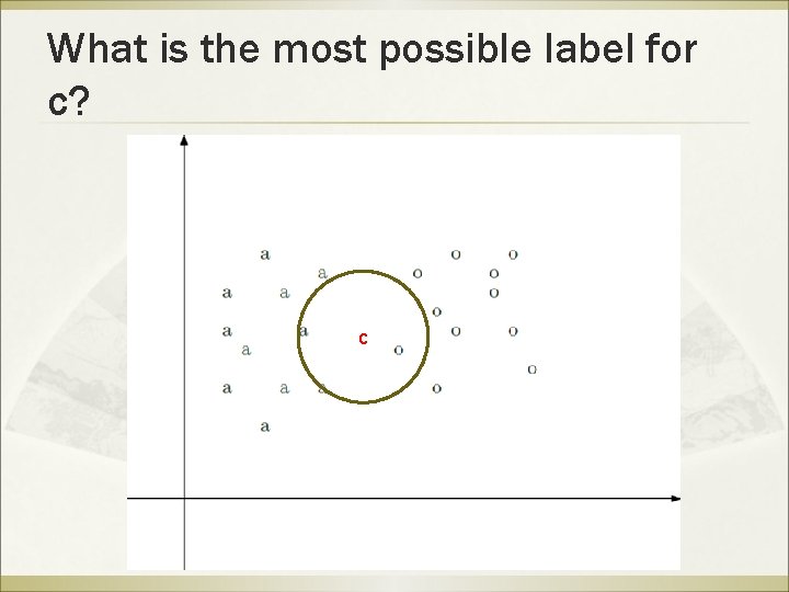
What is the most possible label for c? ß ß ß Solution: Looking for the nearest K neighbors of c. Take the majority label as c’s label Let’s suppose k = 3:

What is the most possible label for c? c

What is the most possible label for c? ß ß The 3 nearest points to c are: a, a and o. Therefore, the most possible label for c is a.

Voronoi Diagram

Voronoi Diagram

Remarks

Choosing the most suitable K

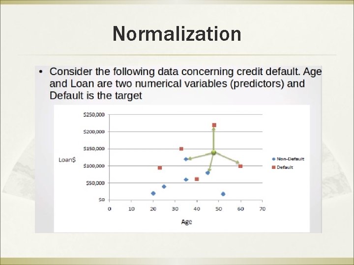
Normalization

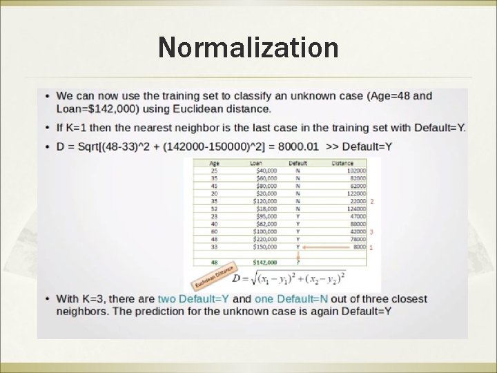
Normalization

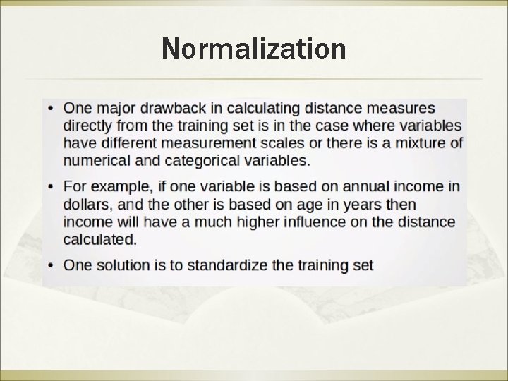
Normalization

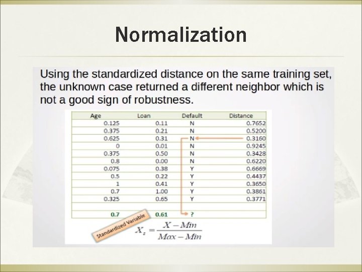
Normalization

k-Nearest Neighbor Classification (k. NN) ß ß ß Unlike all the previous learning methods, k. NN does not build model from the training data. To classify a test instance d, define kneighborhood P as k nearest neighbors of d Count number n of training instances in P that belong to class cj Estimate Pr(cj|d) as n/k No training is needed. Classification time is linear in training set size for each test case. 109

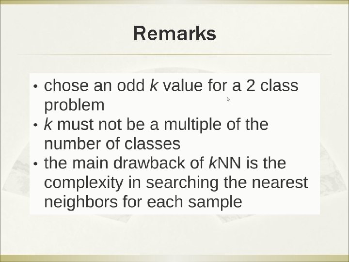
Discussions ß ß k. NN can deal with complex and arbitrary decision boundaries. Despite its simplicity, researchers have shown that the classification accuracy of k. NN can be quite strong and in many cases as accurate as those elaborated methods. k. NN is slow at the classification time k. NN does not produce an understandable model 110

Supervised Learning Methods Frequency Table Covariance Matrix Classificati on Similarity Function Others Bayesian Methods Decision Trees Linear Dis. Analysis Logistic Regression K Nearest Neighbor Neural Network Support Vector Machine

Introduction ß ß ß Support vector machines were invented by V. Vapnik and his co-workers in 1970 s in Russia and became known to the West in 1992. SVMs are linear classifiers that find a hyperplane to separate two class of data, positive and negative. Kernel functions are used for nonlinear separation. SVM not only has a rigorous theoretical foundation, but also performs classification more accurately than most other methods in applications, especially for high dimensional data. It is perhaps the best classifier for text classification. 112

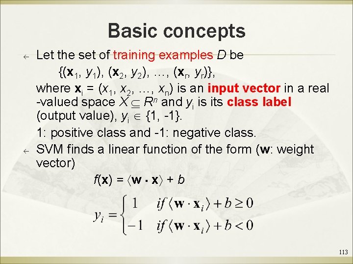
Basic concepts ß ß Let the set of training examples D be {(x 1, y 1), (x 2, y 2), …, (xr, yr)}, where xi = (x 1, x 2, …, xn) is an input vector in a real -valued space X Rn and yi is its class label (output value), yi {1, -1}. 1: positive class and -1: negative class. SVM finds a linear function of the form (w: weight vector) f(x) = w x + b 113

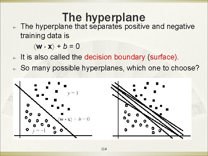
The hyperplane ß ß ß The hyperplane that separates positive and negative training data is w x + b = 0 It is also called the decision boundary (surface). So many possible hyperplanes, which one to choose? 114

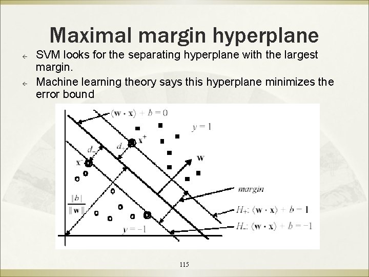
Maximal margin hyperplane ß ß SVM looks for the separating hyperplane with the largest margin. Machine learning theory says this hyperplane minimizes the error bound 115

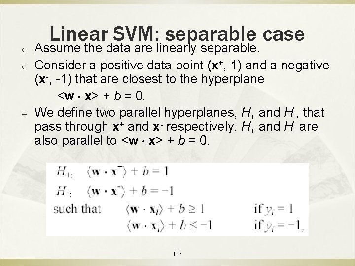
Linear SVM: separable case ß ß ß Assume the data are linearly separable. Consider a positive data point (x+, 1) and a negative (x-, -1) that are closest to the hyperplane <w x> + b = 0. We define two parallel hyperplanes, H+ and H-, that pass through x+ and x- respectively. H+ and H- are also parallel to <w x> + b = 0. 116

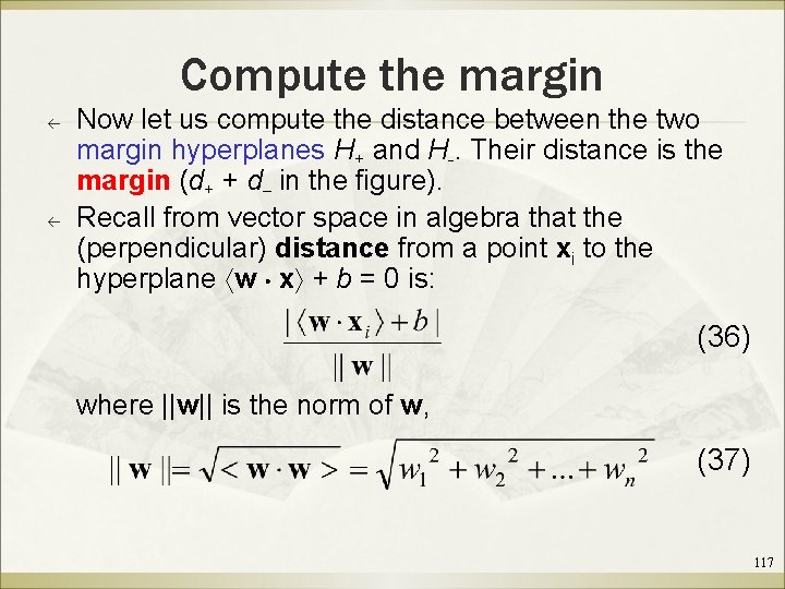
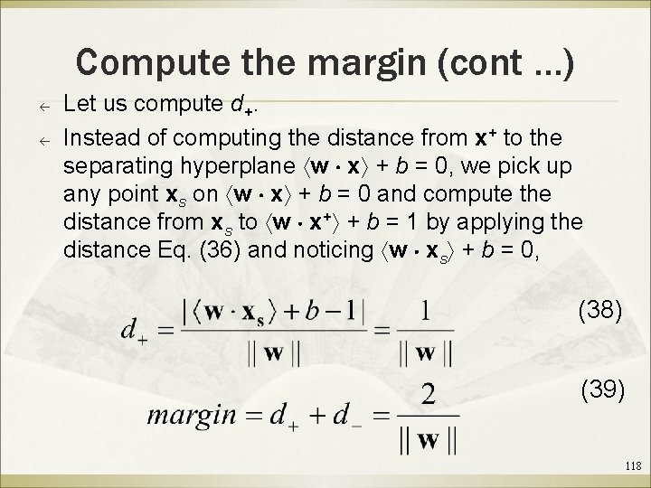
Compute the margin ß ß Now let us compute the distance between the two margin hyperplanes H+ and H-. Their distance is the margin (d+ + d in the figure). Recall from vector space in algebra that the (perpendicular) distance from a point xi to the hyperplane w x + b = 0 is: (36) where ||w|| is the norm of w, (37) 117

Compute the margin (cont …) ß ß Let us compute d+. Instead of computing the distance from x+ to the separating hyperplane w x + b = 0, we pick up any point xs on w x + b = 0 and compute the distance from xs to w x+ + b = 1 by applying the distance Eq. (36) and noticing w xs + b = 0, (38) (39) 118

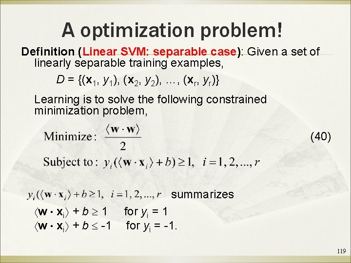
A optimization problem! Definition (Linear SVM: separable case): Given a set of linearly separable training examples, D = {(x 1, y 1), (x 2, y 2), …, (xr, yr)} Learning is to solve the following constrained minimization problem, (40) summarizes w xi + b 1 for yi = 1 w xi + b -1 for yi = -1. 119

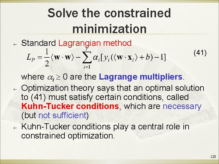
Solve the constrained minimization ß Standard Lagrangian method (41) ß ß where i 0 are the Lagrange multipliers. Optimization theory says that an optimal solution to (41) must satisfy certain conditions, called Kuhn-Tucker conditions, which are necessary (but not sufficient) Kuhn-Tucker conditions play a central role in constrained optimization. 120

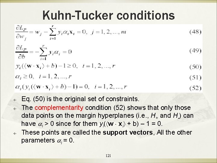
Kuhn-Tucker conditions ß ß ß Eq. (50) is the original set of constraints. The complementarity condition (52) shows that only those data points on the margin hyperplanes (i. e. , H+ and H-) can have i > 0 since for them yi( w xi + b) – 1 = 0. These points are called the support vectors, All the other parameters i = 0. 121

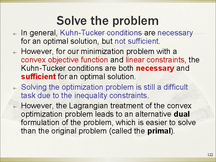
Solve the problem ß ß In general, Kuhn-Tucker conditions are necessary for an optimal solution, but not sufficient. However, for our minimization problem with a convex objective function and linear constraints, the Kuhn-Tucker conditions are both necessary and sufficient for an optimal solution. Solving the optimization problem is still a difficult task due to the inequality constraints. However, the Lagrangian treatment of the convex optimization problem leads to an alternative dual formulation of the problem, which is easier to solve than the original problem (called the primal). 122

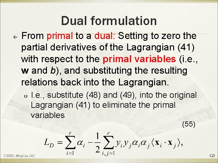
Dual formulation ß From primal to a dual: Setting to zero the partial derivatives of the Lagrangian (41) with respect to the primal variables (i. e. , w and b), and substituting the resulting relations back into the Lagrangian. Þ I. e. , substitute (48) and (49), into the original Lagrangian (41) to eliminate the primal variables (55) CS 583, Bing Liu, UIC 123

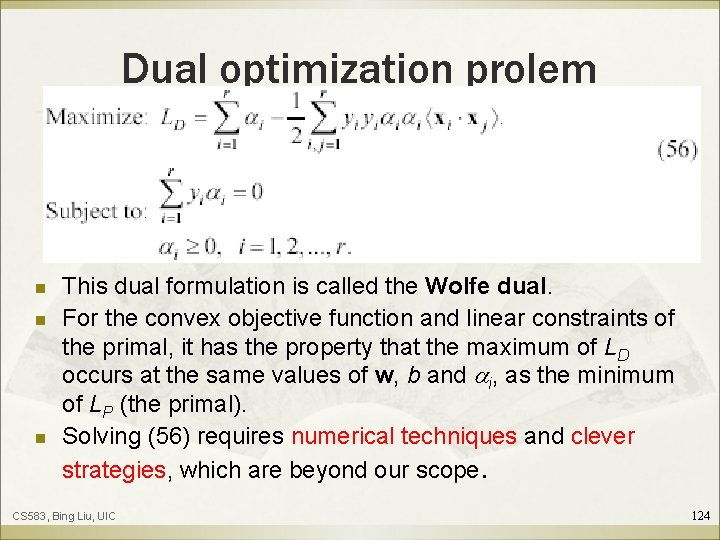
Dual optimization prolem n n n This dual formulation is called the Wolfe dual. For the convex objective function and linear constraints of the primal, it has the property that the maximum of LD occurs at the same values of w, b and i, as the minimum of LP (the primal). Solving (56) requires numerical techniques and clever strategies, which are beyond our scope. CS 583, Bing Liu, UIC 124

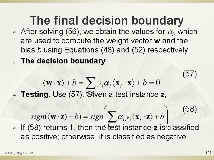
The final decision boundary ß ß After solving (56), we obtain the values for i, which are used to compute the weight vector w and the bias b using Equations (48) and (52) respectively. The decision boundary (57) ß Testing: Use (57). Given a test instance z, (58) ß If (58) returns 1, then the test instance z is classified as positive; otherwise, it is classified as negative. CS 583, Bing Liu, UIC 125

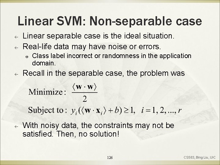
Linear SVM: Non-separable case ß ß Linear separable case is the ideal situation. Real-life data may have noise or errors. Þ ß ß Class label incorrect or randomness in the application domain. Recall in the separable case, the problem was With noisy data, the constraints may not be satisfied. Then, no solution! 126 CS 583, Bing Liu, UIC

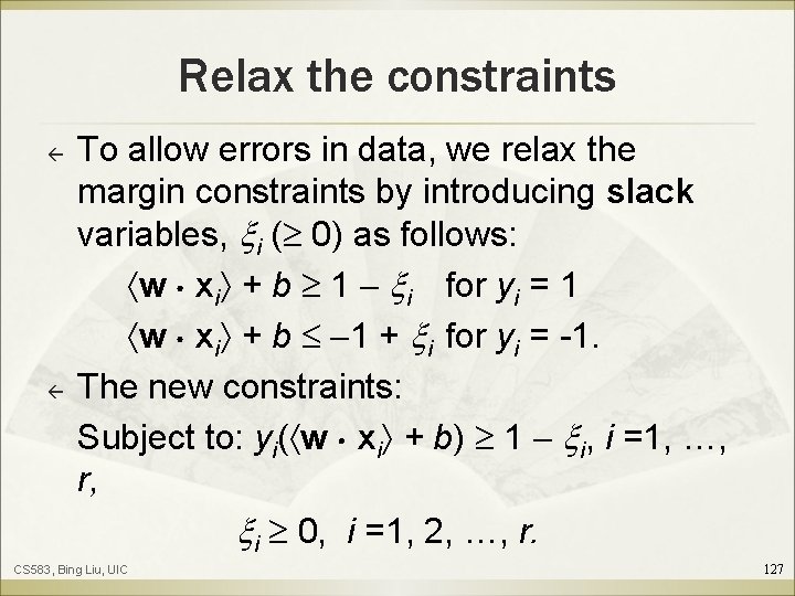
Relax the constraints ß ß To allow errors in data, we relax the margin constraints by introducing slack variables, i ( 0) as follows: w xi + b 1 i for yi = 1 w xi + b 1 + i for yi = -1. The new constraints: Subject to: yi( w xi + b) 1 i, i =1, …, r, i 0, i =1, 2, …, r. CS 583, Bing Liu, UIC 127

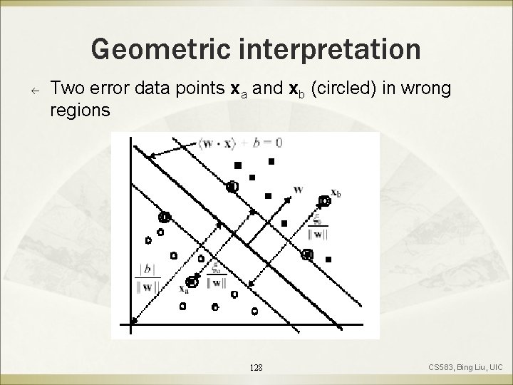
Geometric interpretation ß Two error data points xa and xb (circled) in wrong regions 128 CS 583, Bing Liu, UIC

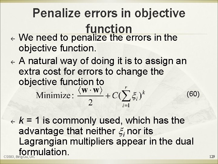
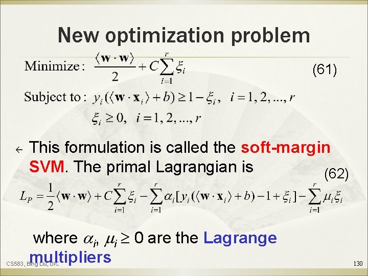
Penalize errors in objective function ß ß We need to penalize the errors in the objective function. A natural way of doing it is to assign an extra cost for errors to change the objective function to (60) ß k = 1 is commonly used, which has the advantage that neither i nor its Lagrangian multipliers appear in the dual formulation. CS 583, Bing Liu, UIC 129

New optimization problem (61) ß This formulation is called the soft-margin SVM. The primal Lagrangian is (62) where i, i 0 are the Lagrange multipliers CS 583, Bing Liu, UIC 130

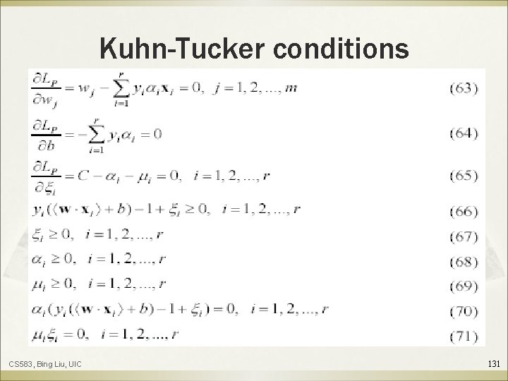
Kuhn-Tucker conditions CS 583, Bing Liu, UIC 131

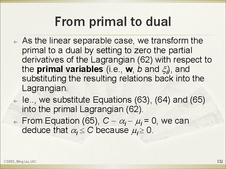
From primal to dual ß ß ß As the linear separable case, we transform the primal to a dual by setting to zero the partial derivatives of the Lagrangian (62) with respect to the primal variables (i. e. , w, b and i), and substituting the resulting relations back into the Lagrangian. Ie. . , we substitute Equations (63), (64) and (65) into the primal Lagrangian (62). From Equation (65), C i i = 0, we can deduce that i C because i 0. CS 583, Bing Liu, UIC 132

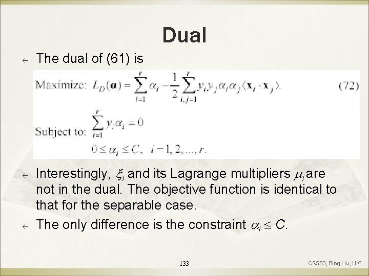
Dual ß ß ß The dual of (61) is Interestingly, i and its Lagrange multipliers i are not in the dual. The objective function is identical to that for the separable case. The only difference is the constraint i C. 133 CS 583, Bing Liu, UIC

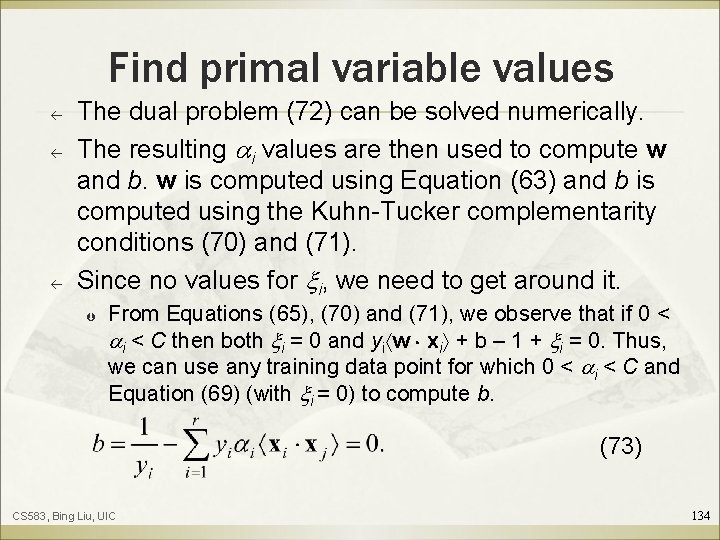
Find primal variable values ß ß ß The dual problem (72) can be solved numerically. The resulting i values are then used to compute w and b. w is computed using Equation (63) and b is computed using the Kuhn-Tucker complementarity conditions (70) and (71). Since no values for i, we need to get around it. Þ From Equations (65), (70) and (71), we observe that if 0 < i < C then both i = 0 and yi w xi + b – 1 + i = 0. Thus, we can use any training data point for which 0 < i < C and Equation (69) (with i = 0) to compute b. (73) CS 583, Bing Liu, UIC 134

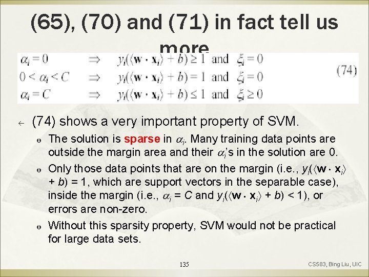
(65), (70) and (71) in fact tell us more ß (74) shows a very important property of SVM. Þ Þ Þ The solution is sparse in i. Many training data points are outside the margin area and their i’s in the solution are 0. Only those data points that are on the margin (i. e. , yi( w xi + b) = 1, which are support vectors in the separable case), inside the margin (i. e. , i = C and yi( w xi + b) < 1), or errors are non-zero. Without this sparsity property, SVM would not be practical for large data sets. 135 CS 583, Bing Liu, UIC

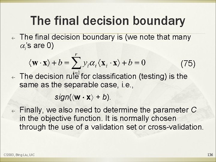
The final decision boundary ß The final decision boundary is (we note that many i’s are 0) (75) ß The decision rule for classification (testing) is the same as the separable case, i. e. , sign( w x + b). ß Finally, we also need to determine the parameter C in the objective function. It is normally chosen through the use of a validation set or cross-validation. CS 583, Bing Liu, UIC 136

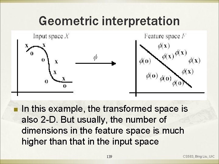
ß ß ß How to deal with nonlinear separation? The SVM formulations require linear separation. Real-life data sets may need nonlinear separation. To deal with nonlinear separation, the same formulation and techniques as for the linear case are still used. We only transform the input data into another space (usually of a much higher dimension) so that Þ a linear decision boundary can separate positive and negative examples in the transformed space, The transformed space is called the feature space. The original data space is called the input space. CS 583, Bing Liu, UIC 137

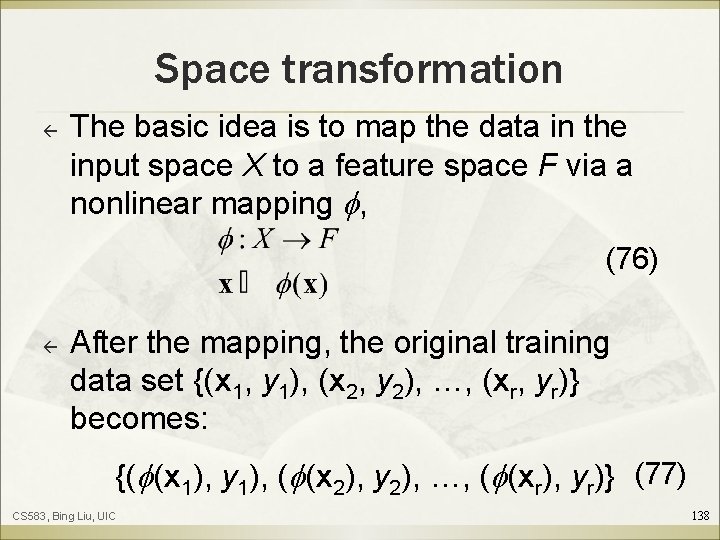
Space transformation ß The basic idea is to map the data in the input space X to a feature space F via a nonlinear mapping , (76) ß After the mapping, the original training data set {(x 1, y 1), (x 2, y 2), …, (xr, yr)} becomes: {( (x 1), y 1), ( (x 2), y 2), …, ( (xr), yr)} (77) CS 583, Bing Liu, UIC 138

Geometric interpretation n In this example, the transformed space is also 2 -D. But usually, the number of dimensions in the feature space is much higher than that in the input space 139 CS 583, Bing Liu, UIC

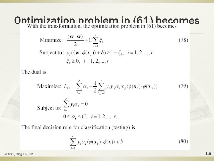
Optimization problem in (61) becomes CS 583, Bing Liu, UIC 140

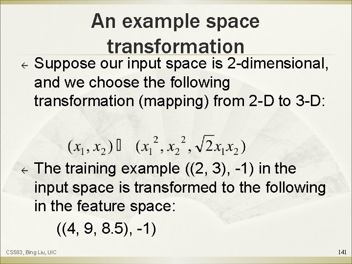
An example space transformation ß ß Suppose our input space is 2 -dimensional, and we choose the following transformation (mapping) from 2 -D to 3 -D: The training example ((2, 3), -1) in the input space is transformed to the following in the feature space: ((4, 9, 8. 5), -1) CS 583, Bing Liu, UIC 141

Problem with explicit transformation ß ß The potential problem with this explicit data transformation and then applying the linear SVM is that it may suffer from the curse of dimensionality. The number of dimensions in the feature space can be huge with some useful transformations even with reasonable numbers of attributes in the input space. This makes it computationally infeasible to handle. Fortunately, explicit transformation is not needed. CS 583, Bing Liu, UIC 142

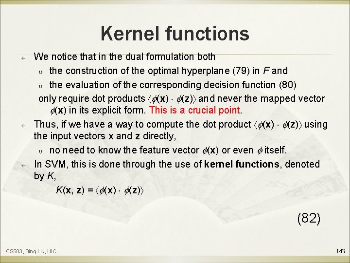
Kernel functions ß ß ß We notice that in the dual formulation both Þ the construction of the optimal hyperplane (79) in F and Þ the evaluation of the corresponding decision function (80) only require dot products (x) (z) and never the mapped vector (x) in its explicit form. This is a crucial point. Thus, if we have a way to compute the dot product (x) (z) using the input vectors x and z directly, Þ no need to know the feature vector (x) or even itself. In SVM, this is done through the use of kernel functions, denoted by K, K(x, z) = (x) (z) (82) CS 583, Bing Liu, UIC 143

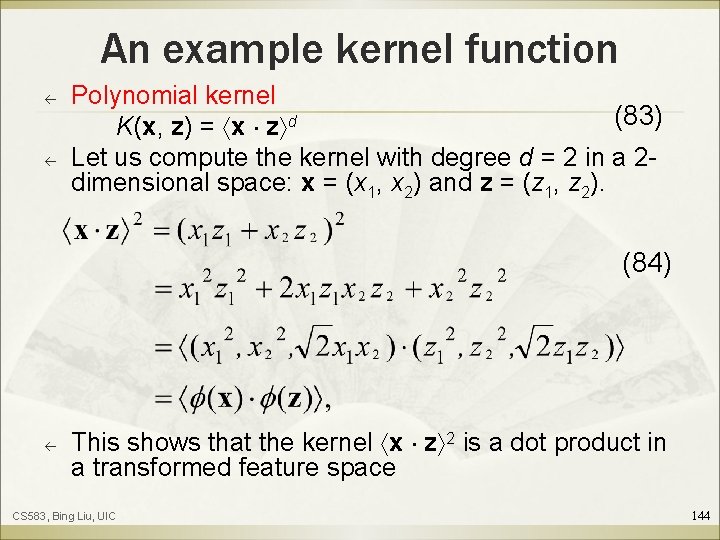
An example kernel function ß ß Polynomial kernel (83) K(x, z) = x z d Let us compute the kernel with degree d = 2 in a 2 dimensional space: x = (x 1, x 2) and z = (z 1, z 2). (84) ß This shows that the kernel x z 2 is a dot product in a transformed feature space CS 583, Bing Liu, UIC 144

Kernel trick ß ß ß The derivation in (84) is only for illustration purposes. We do not need to find the mapping function. We can simply apply the kernel function directly by Þ ß replace all the dot products (x) (z) in (79) and (80) with the kernel function K(x, z) (e. g. , the polynomial kernel x z d in (83)). This strategy is called the kernel trick. CS 583, Bing Liu, UIC 145

Is it a kernel function? ß The question is: how do we know whether a function is a kernel without performing the derivation such as that in (84)? I. e, Þ ß How do we know that a kernel function is indeed a dot product in some feature space? This question is answered by a theorem called the Mercer’s theorem, which we will not discuss here. CS 583, Bing Liu, UIC 146

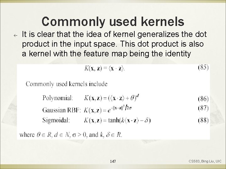
Commonly used kernels ß It is clear that the idea of kernel generalizes the dot product in the input space. This dot product is also a kernel with the feature map being the identity 147 CS 583, Bing Liu, UIC

Some other issues in SVM ß ß ß SVM works only in a real-valued space. For a categorical attribute, we need to convert its categorical values to numeric values. SVM does only two-classification. For multiclass problems, some strategies can be applied, e. g. , one-against-rest, and error-correcting output coding. The hyperplane produced by SVM is hard to understand by human users. The matter is made worse by kernels. Thus, SVM is commonly used in applications that do not required human understanding. 148

Summary ß ß ß Applications of supervised learning are in almost any field or domain. We studied 4 classification techniques. There are still many other methods, e. g. , Bayesian networks Þ Neural networks Þ Genetic algorithms Þ Fuzzy classification This large number of methods also show the importance of classification and its wide applicability. Þ ß It remains to be an active research area. CS 583, Bing Liu, UIC 149