Classification Logistic Regression maybe deep learning Slides by

Classification & Logistic Regression & maybe deep learning Slides by: Joseph E. Gonzalez jegonzal@cs. berkeley. edu ?

Previously…

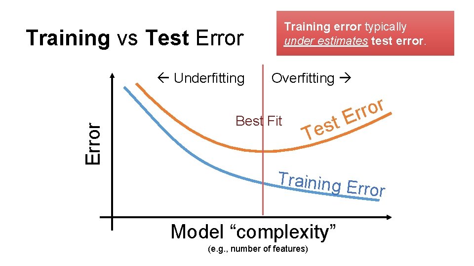
Training error typically under estimates test error. Training vs Test Error Underfitting Overfitting Best Fit t s Te r o r Er Training E rror Model “complexity” (e. g. , number of features)

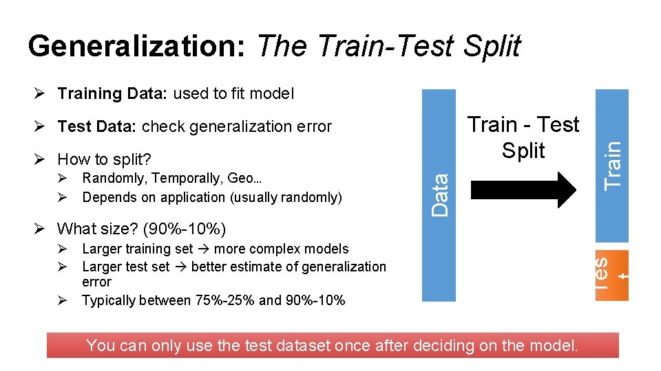
Generalization: The Train-Test Split Train - Test Split Ø Test Data: check generalization error Ø Randomly, Temporally, Geo… Ø Depends on application (usually randomly) Data Ø How to split? Train Ø Training Data: used to fit model Ø Larger training set more complex models Ø Larger test set better estimate of generalization error Ø Typically between 75%-25% and 90%-10% You can only use the test dataset once after deciding on the model. Tes t Ø What size? (90%-10%)

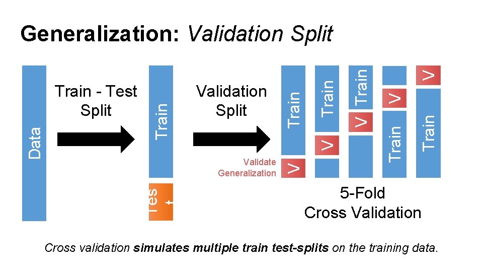
V Train V V Train Validation Split Validate Generalization Tes t Data Train - Test Split Train Generalization: Validation Split 5 -Fold Cross Validation Cross validation simulates multiple train test-splits on the training data.

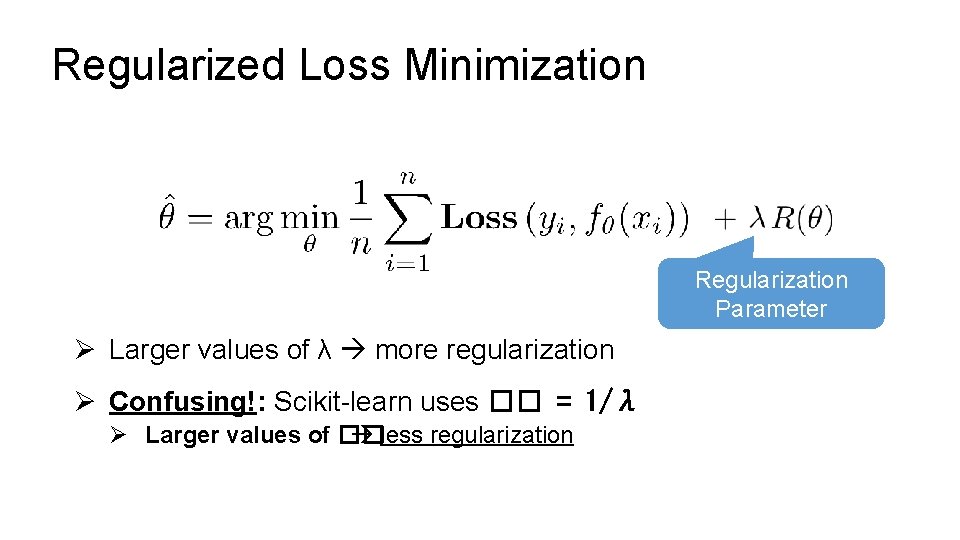
Regularized Loss Minimization Regularization Parameter Ø Larger values of λ more regularization Ø Confusing!: Scikit-learn uses �� = 1/λ Ø Larger values of �� less regularization

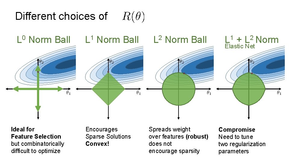
Different choices of L 0 Norm Ball Ideal for Feature Selection but combinatorically difficult to optimize L 1 Norm Ball Encourages Sparse Solutions Convex! L 2 Norm Ball Spreads weight over features (robust) does not encourage sparsity L 1 + L 2 Norm Elastic Net Compromise Need to tune two regularization parameters

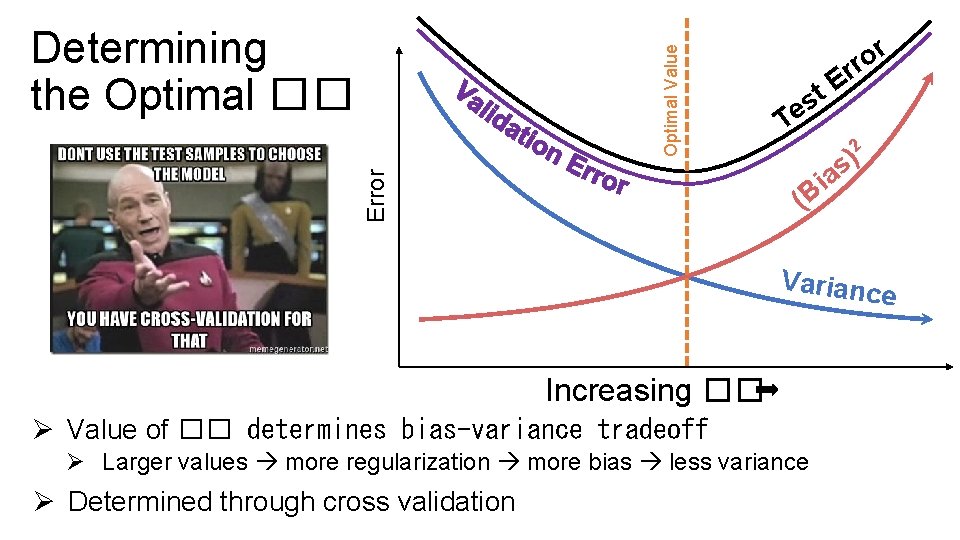
r o rr T E t es Varianc e Increasing �� Ø Value of �� determines bias-variance tradeoff Ø Larger values more regularization more bias less variance Ø Determined through cross validation 2 ) as i B ( Error How do we determine ��? Optimal Value Determining the Optimal ��

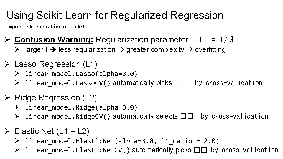
Using Scikit-Learn for Regularized Regression import sklearn. linear_model Ø Confusion Warning: Regularization parameter �� = 1/λ Ø larger �� less regularization greater complexity overfitting Ø Lasso Regression (L 1) Ø linear_model. Lasso(alpha=3. 0) Ø linear_model. Lasso. CV() automatically picks �� by cross-validation Ø Ridge Regression (L 2) Ø linear_model. Ridge(alpha=3. 0) Ø linear_model. Ridge. CV() automatically selects �� by cross-validation Ø Elastic Net (L 1 + L 2) Ø linear_model. Elastic. Net(alpha=3. 0, l 1_ratio = 2. 0) Ø linear_model. Elastic. Net. CV() automatically picks �� by cross-validation

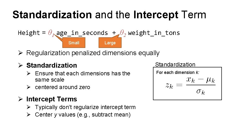
Standardization and the Intercept Term Height = θ 1 age_in_seconds + θ 2 weight_in_tons Small Large Ø Regularization penalized dimensions equally Ø Standardization Ø Ensure that each dimensions has the same scale Ø centered around zero Ø Intercept Terms Ø Typically don’t regularize intercept term Ø Center y values (e. g. , subtract mean) Standardization For each dimension k:

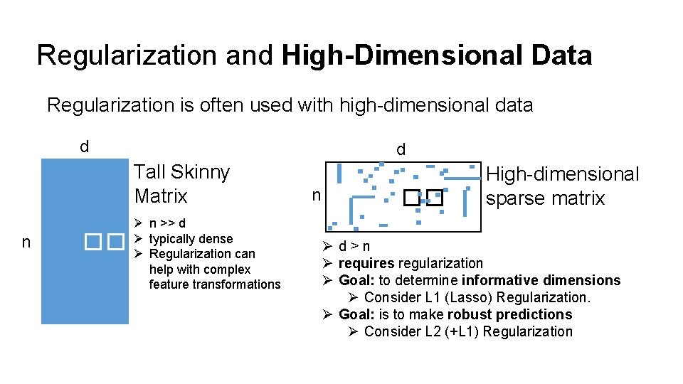
Regularization and High-Dimensional Data Regularization is often used with high-dimensional data d d Tall Skinny Matrix n �� Ø n >> d Ø typically dense Ø Regularization can help with complex feature transformations n �� High-dimensional sparse matrix Ød>n Ø requires regularization Ø Goal: to determine informative dimensions Ø Consider L 1 (Lasso) Regularization. Ø Goal: is to make robust predictions Ø Consider L 2 (+L 1) Regularization

Today Classification

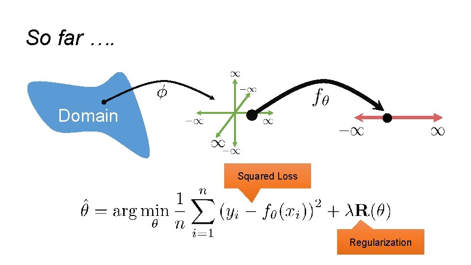
So far …. Domain Squared Loss Regularization

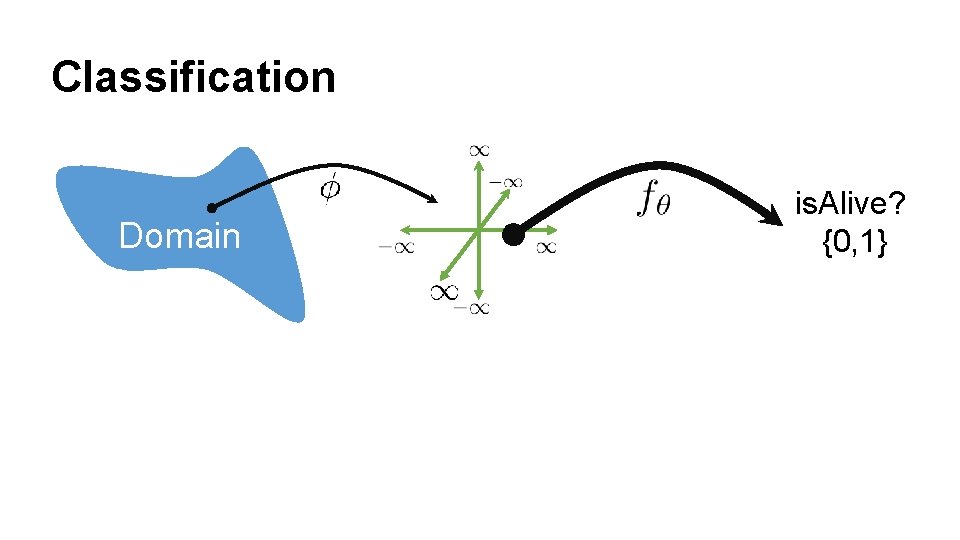
Classification Domain is. Alive? {0, 1}

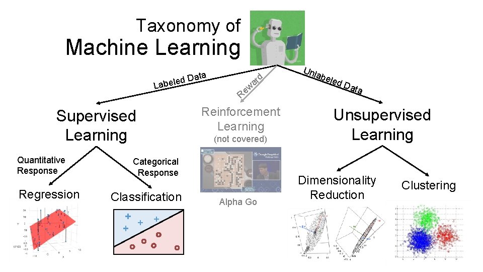
Taxonomy of Machine Learning ta ed Da Label Supervised Learning Quantitative Response Regression d ar w Re Reinforcement Learning (not covered) Categorical Response Classification Alpha Go Unl abe led Dat a Unsupervised Learning Dimensionality Reduction Clustering

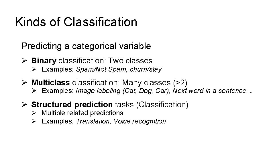
Kinds of Classification Predicting a categorical variable Ø Binary classification: Two classes Ø Examples: Spam/Not Spam, churn/stay Ø Multiclassification: Many classes (>2) Ø Examples: Image labeling (Cat, Dog, Car), Next word in a sentence … Ø Structured prediction tasks (Classification) Ø Multiple related predictions Ø Examples: Translation, Voice recognition

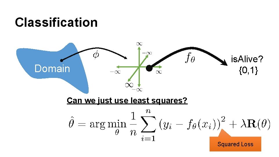
Classification Domain is. Alive? {0, 1} Can we just use least squares? Squared Loss

Python Demo

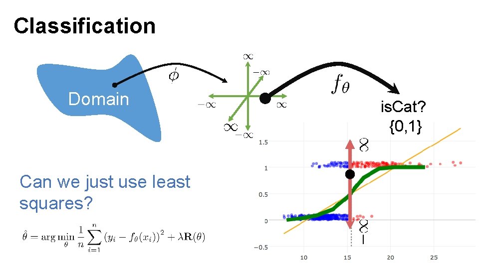
Classification Domain Can we just use least squares? is. Cat? {0, 1}

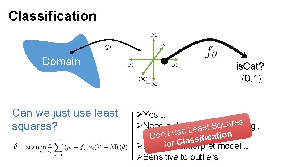
Classification Domain Can we just use least squares? is. Cat? {0, 1} ØYes … s(e. g. , e r a u q ØNeed a decision function S t s a e L e… s u t ’ n n o o f(x) > 0. 5) i t D a c i if s s a l C forto interpret model … ØDifficult ØSensitive to outliers

Defining a New Model for Classification

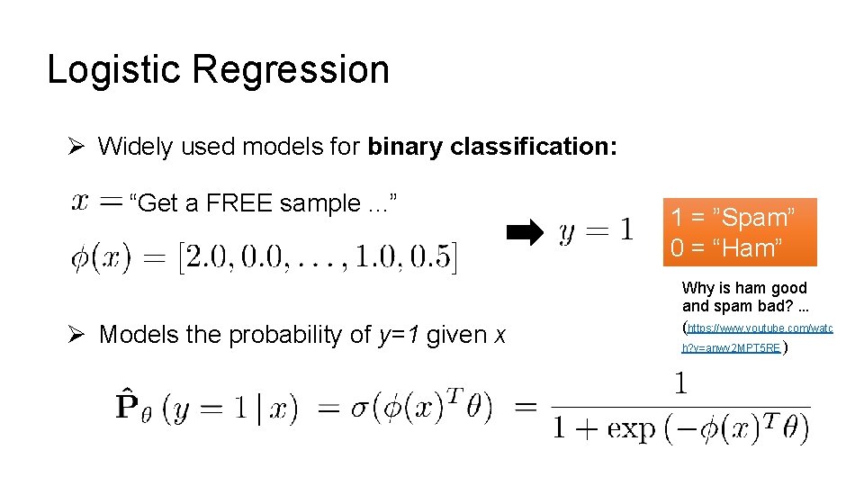
Logistic Regression Ø Widely used models for binary classification: “Get a FREE sample. . . ” Ø Models the probability of y=1 given x 1 = ”Spam” 0 = “Ham” Why is ham good and spam bad? … (https: //www. youtube. com/watc h? v=anwy 2 MPT 5 RE )

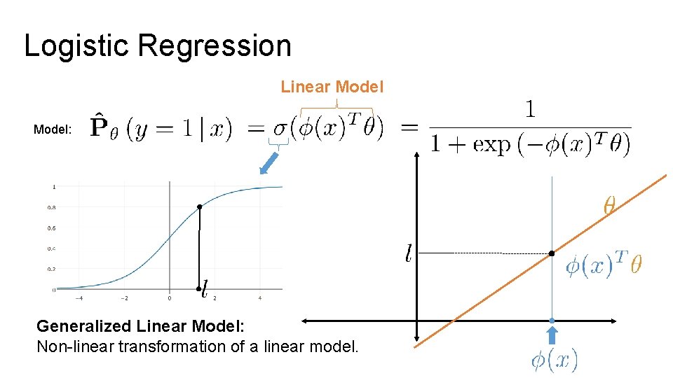
Logistic Regression Linear Model: Generalized Linear Model: Non-linear transformation of a linear model.

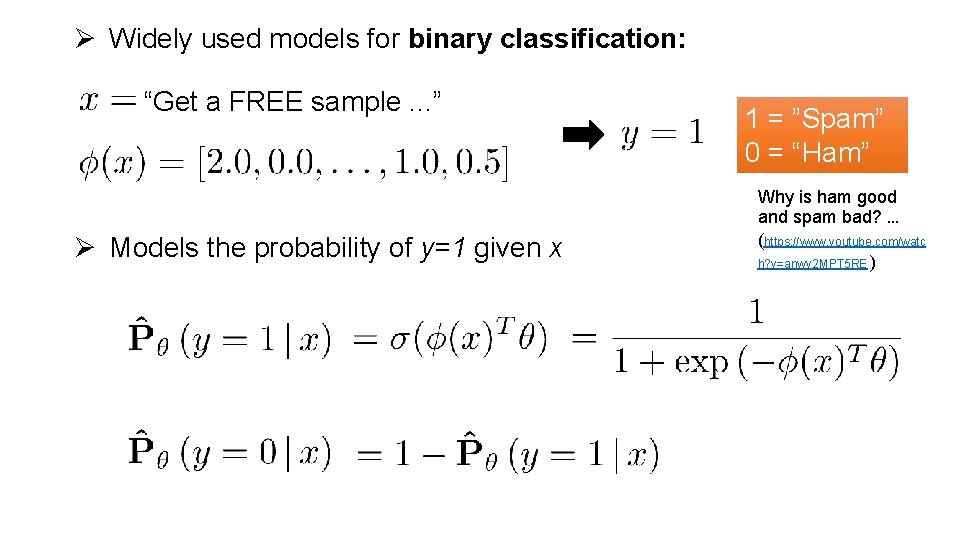
Ø Widely used models for binary classification: “Get a FREE sample. . . ” Ø Models the probability of y=1 given x 1 = ”Spam” 0 = “Ham” Why is ham good and spam bad? … (https: //www. youtube. com/watc h? v=anwy 2 MPT 5 RE )

Python Demo Visualizing the sigmoid (Part 2 notebook)

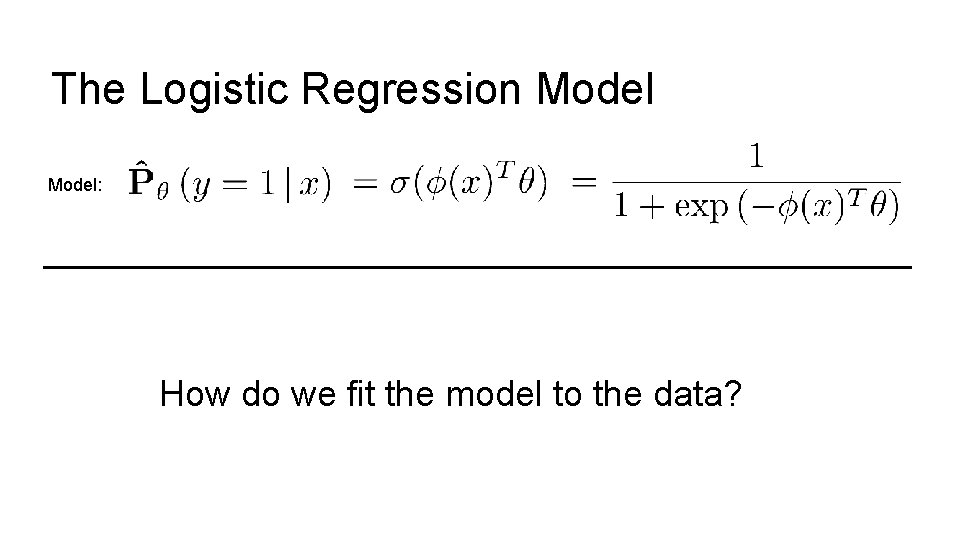
The Logistic Regression Model: How do we fit the model to the data?

Defining the Loss

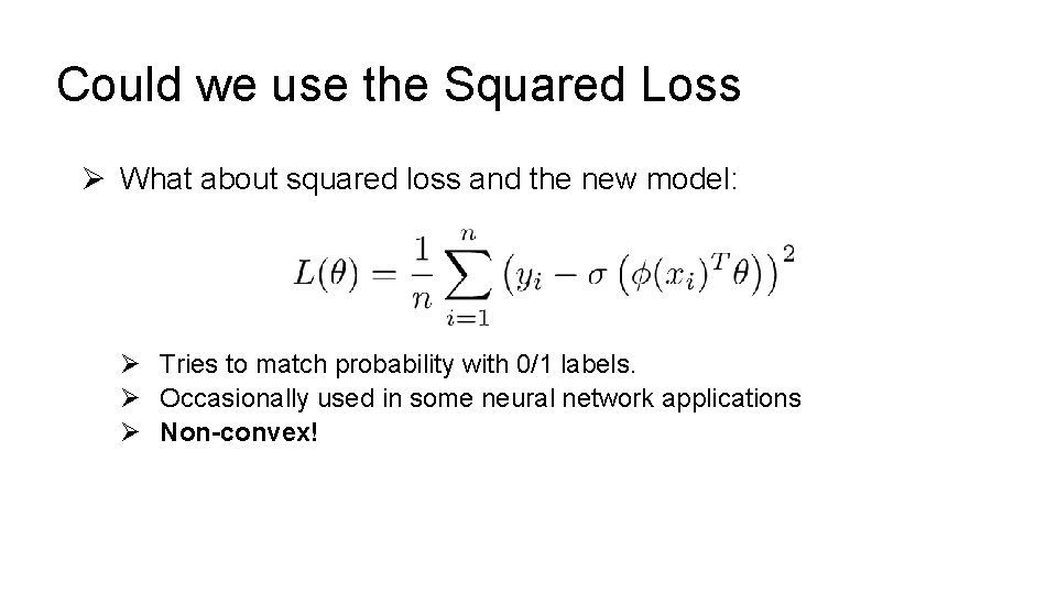
Could we use the Squared Loss Ø What about squared loss and the new model: Ø Tries to match probability with 0/1 labels. Ø Occasionally used in some neural network applications Ø Non-convex!

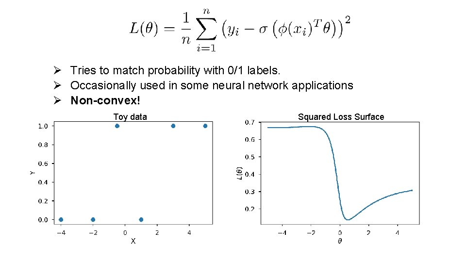
Ø Tries to match probability with 0/1 labels. Ø Occasionally used in some neural network applications Ø Non-convex! Toy data Squared Loss Surface

Defining the Cross Entropy Loss

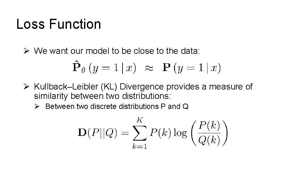
Loss Function Ø We want our model to be close to the data: Ø Kullback–Leibler (KL) Divergence provides a measure of similarity between two distributions: Ø Between two discrete distributions P and Q

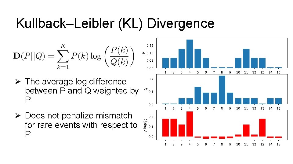
Kullback–Leibler (KL) Divergence Ø The average log difference between P and Q weighted by P Ø Does not penalize mismatch for rare events with respect to P

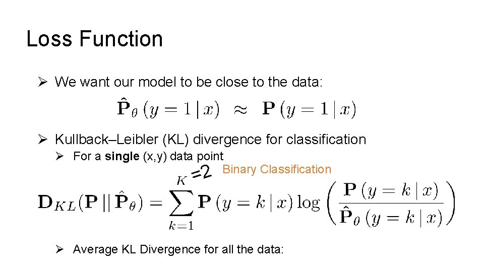
Loss Function Ø We want our model to be close to the data: Ø Kullback–Leibler (KL) divergence for classification Ø For a single (x, y) data point 2 Binary Classification = Ø Average KL Divergence for all the data:

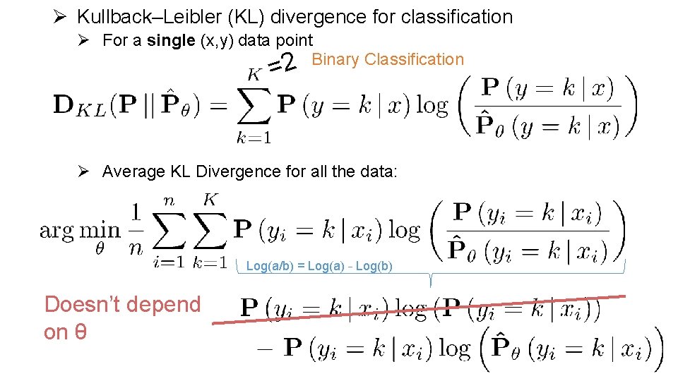
Ø Kullback–Leibler (KL) divergence for classification Ø For a single (x, y) data point 2 Binary Classification = Ø Average KL Divergence for all the data: Log(a/b) = Log(a) – Log(b) Doesn’t depend on θ

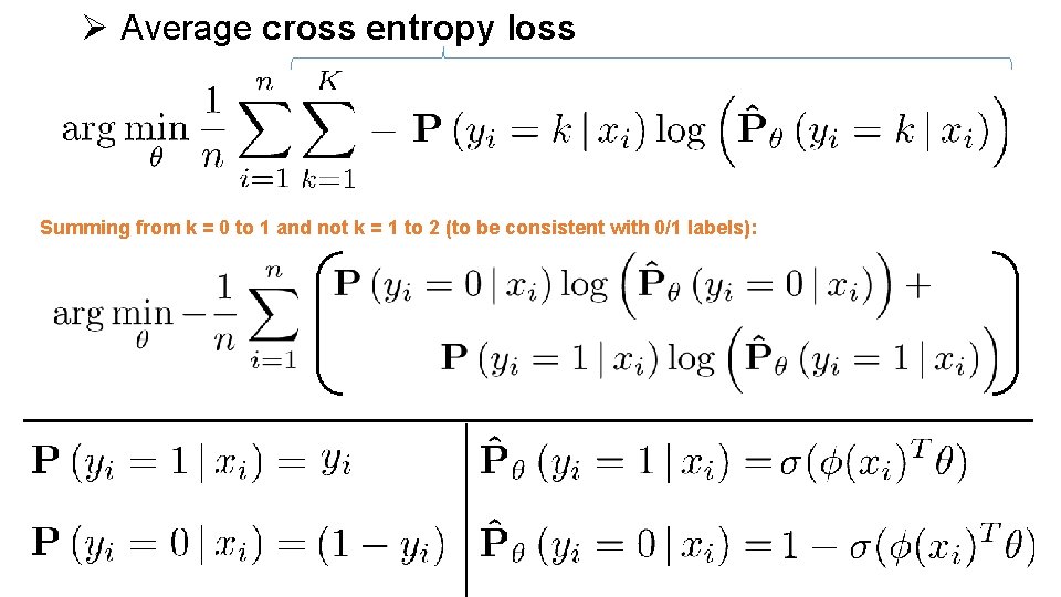
Ø Average cross entropy loss Summing from k = 0 to 1 and not k = 1 to 2 (to be consistent with 0/1 labels):

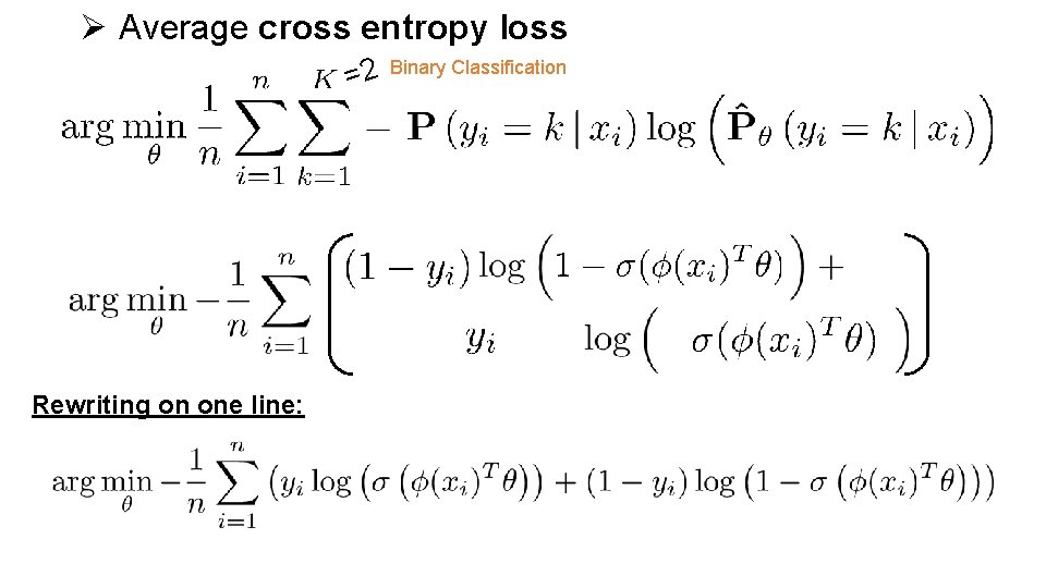
Ø Average cross entropy loss =2 Rewriting on one line: Binary Classification

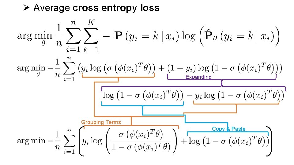
Ø Average cross entropy loss Expanding Grouping Terms Copy & Paste

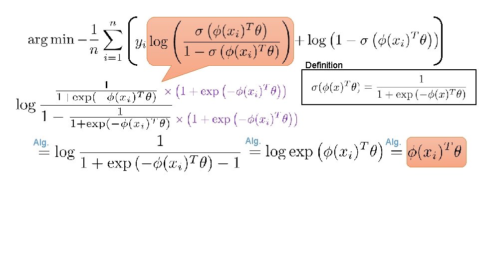
Definition Alg.

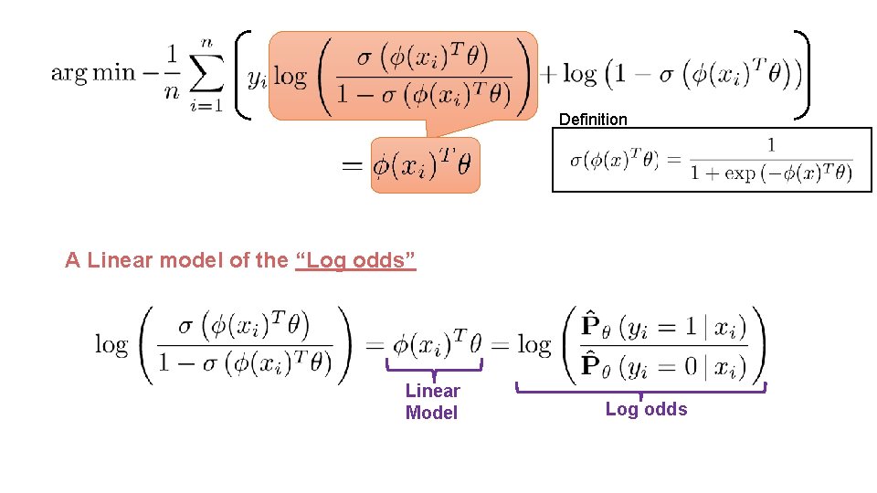
Definition A Linear model of the “Log odds” Linear Model Log odds

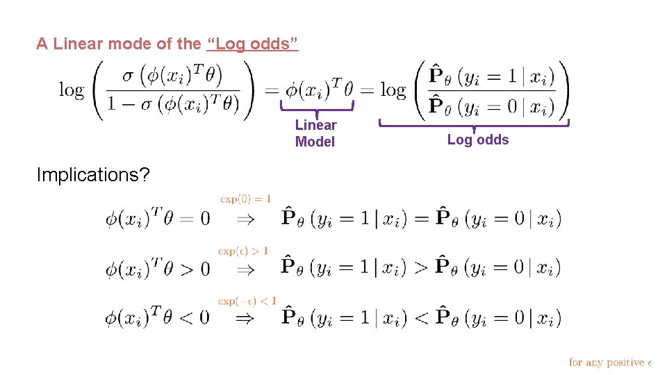
A Linear mode of the “Log odds” Linear Model Implications? Log odds

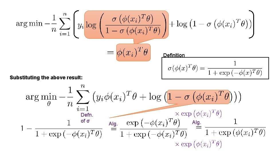
Definition Substituting the above result: Defn. of σ Alg.

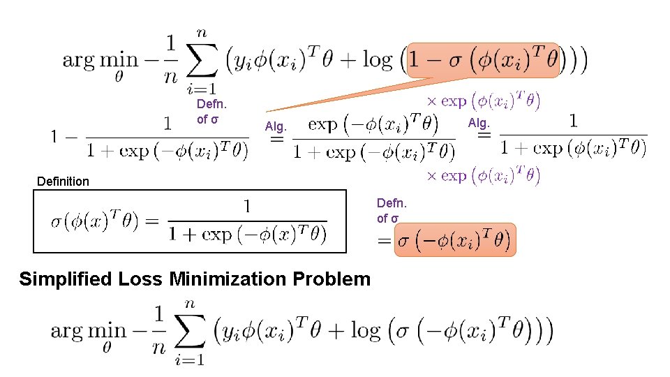
Defn. of σ Alg. Definition Defn. of σ Simplified Loss Minimization Problem

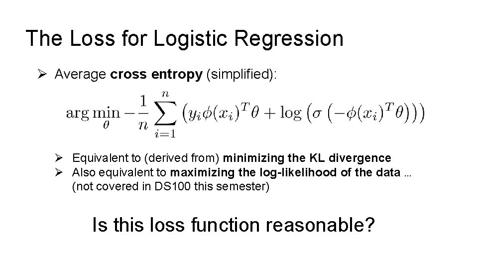
The Loss for Logistic Regression Ø Average cross entropy (simplified): Ø Equivalent to (derived from) minimizing the KL divergence Ø Also equivalent to maximizing the log-likelihood of the data … (not covered in DS 100 this semester) Is this loss function reasonable?

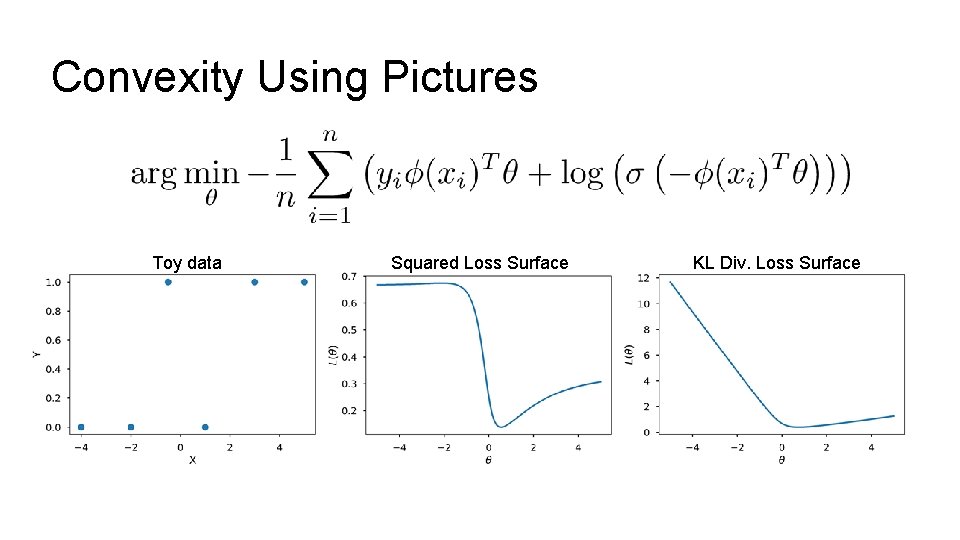
Convexity Using Pictures Toy data Squared Loss Surface KL Div. Loss Surface

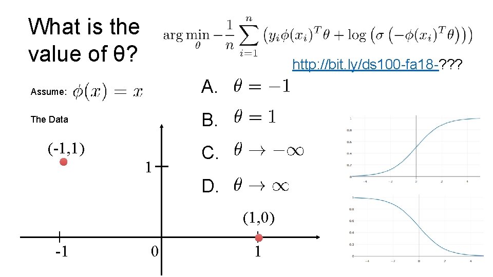
What is the value of θ? http: //bit. ly/ds 100 -fa 18 -? ? ? A. Assume: B. The Data (-1, 1) 1 C. D. (1, 0) -1 0 1

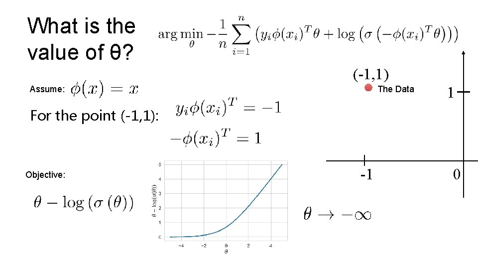
What is the value of θ? (-1, 1) The Data Assume: 1 For the point (-1, 1): Objective: -1 0

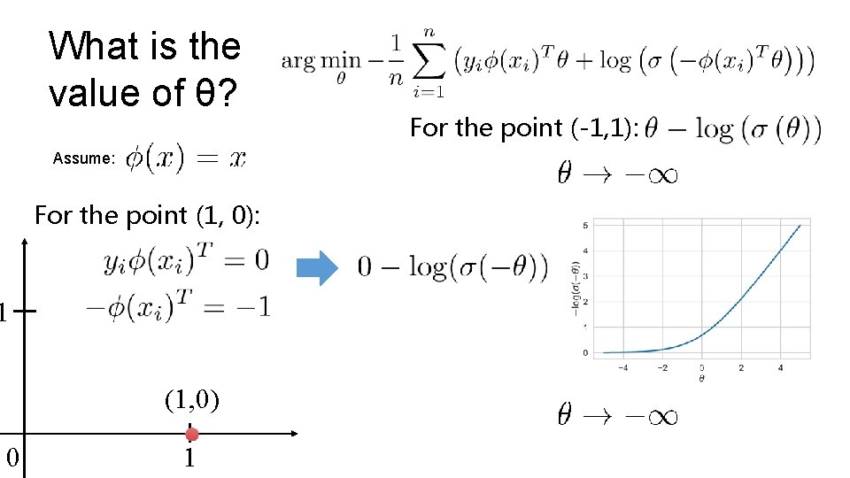
What is the value of θ? Assume: For the point (1, 0): 1 (1, 0) 0 1 For the point (-1, 1):

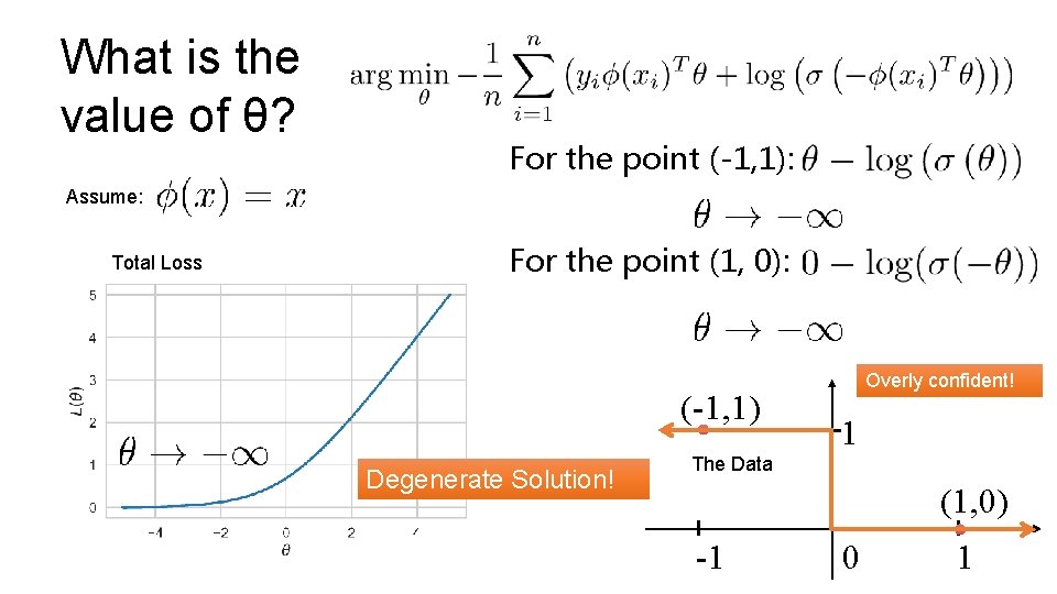
What is the value of θ? For the point (-1, 1): Assume: Total Loss For the point (1, 0): (-1, 1) Degenerate Solution! The Data Overly confident! 1 (1, 0) -1 0 1

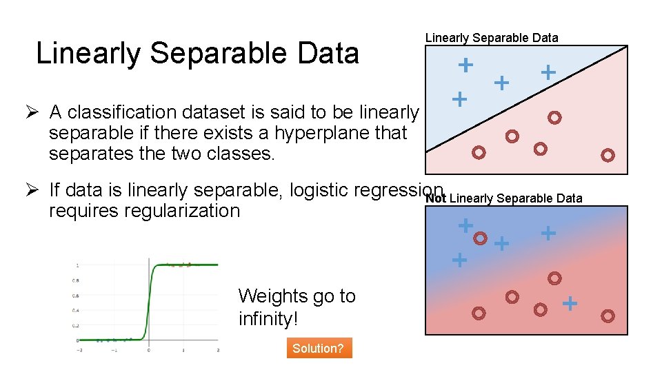
Linearly Separable Data Ø A classification dataset is said to be linearly separable if there exists a hyperplane that separates the two classes. Ø If data is linearly separable, logistic regression Not Linearly Separable Data requires regularization Weights go to infinity! Solution?

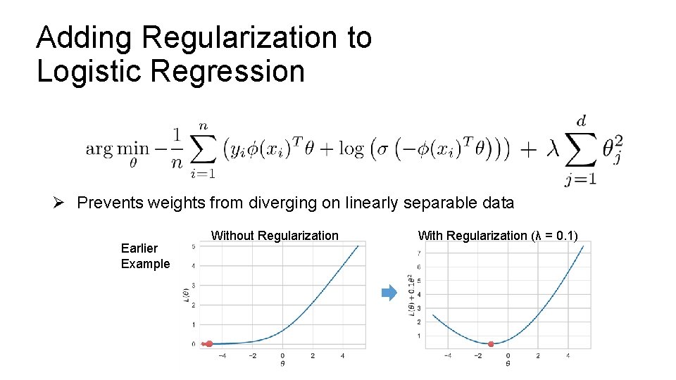
Adding Regularization to Logistic Regression Ø Prevents weights from diverging on linearly separable data Earlier Example Without Regularization With Regularization (λ = 0. 1)

Minimize the Loss

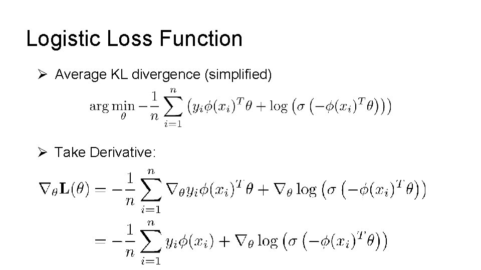
Logistic Loss Function Ø Average KL divergence (simplified) Ø Take Derivative:

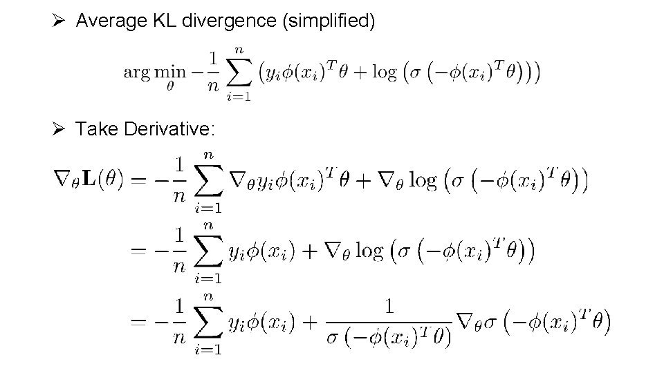
Ø Average KL divergence (simplified) Ø Take Derivative:

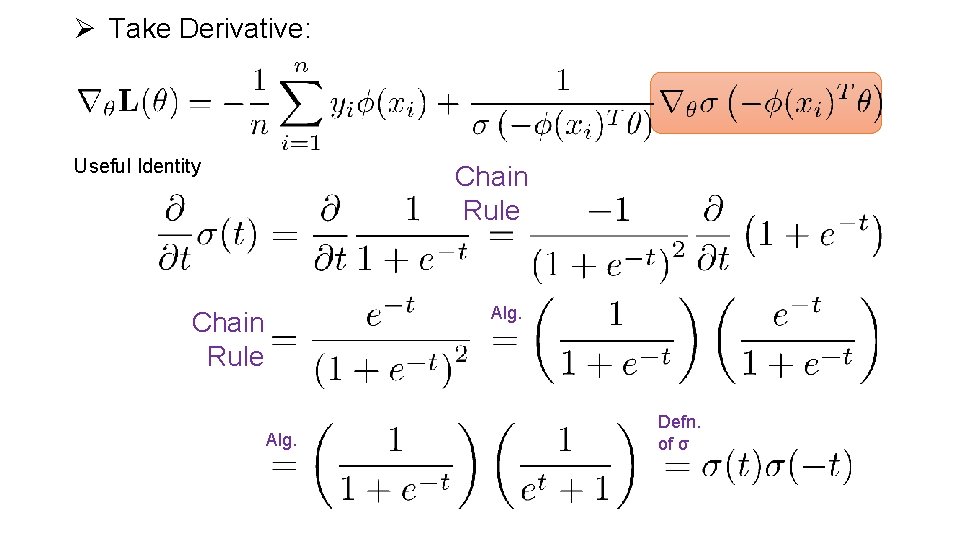
Ø Take Derivative: Useful Identity Chain Rule Alg. Defn. of σ

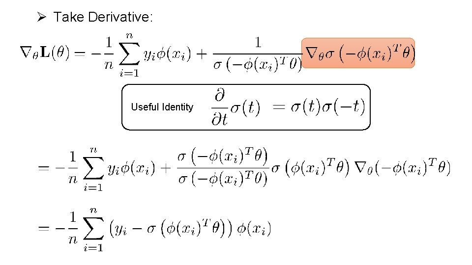
Ø Take Derivative: Useful Identity

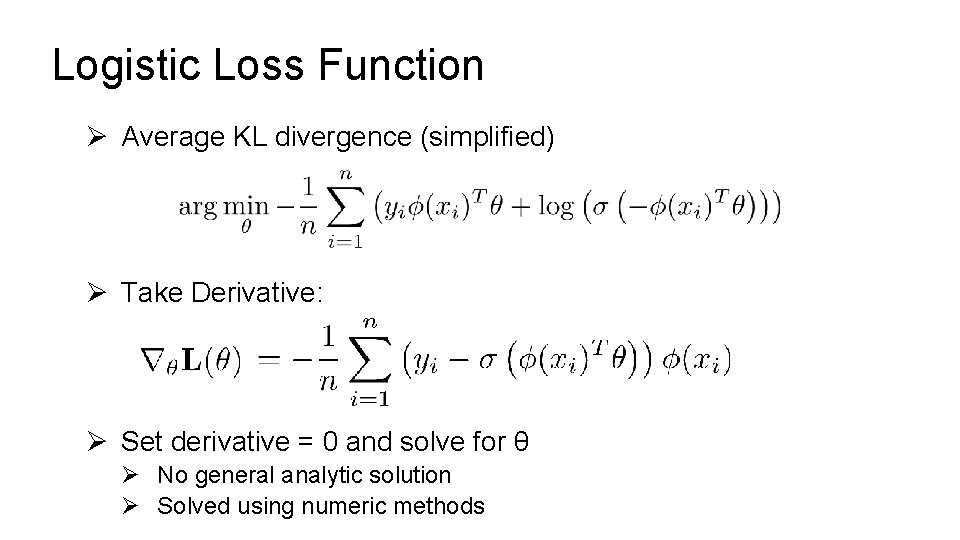
Logistic Loss Function Ø Average KL divergence (simplified) Ø Take Derivative: Ø Set derivative = 0 and solve for θ Ø No general analytic solution Ø Solved using numeric methods

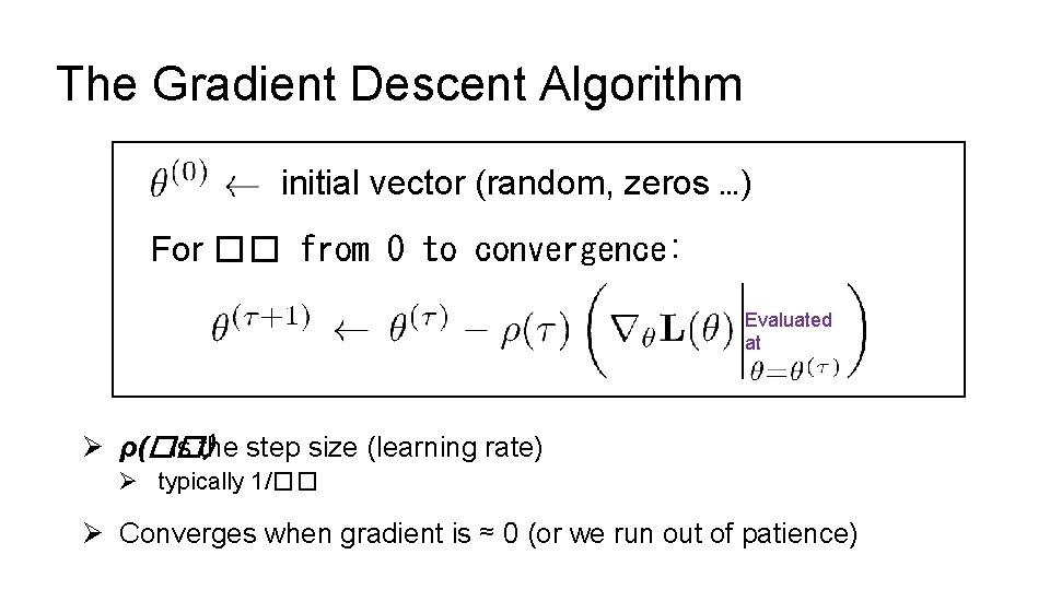
The Gradient Descent Algorithm initial vector (random, zeros …) For �� from 0 to convergence: Evaluated at Ø ρ(��) is the step size (learning rate) Ø typically 1/�� Ø Converges when gradient is ≈ 0 (or we run out of patience)

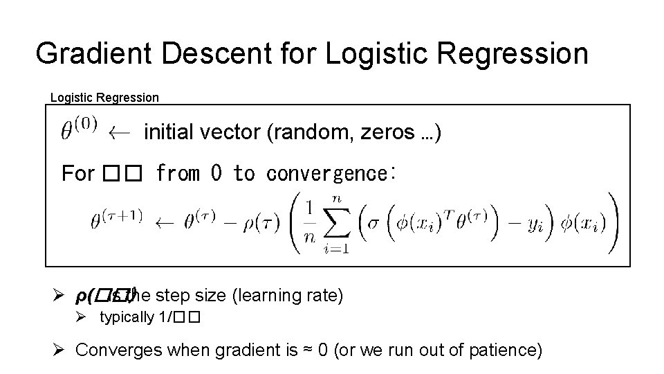
Gradient Descent for Logistic Regression initial vector (random, zeros …) For �� from 0 to convergence: Ø ρ(��) is the step size (learning rate) Ø typically 1/�� Ø Converges when gradient is ≈ 0 (or we run out of patience)

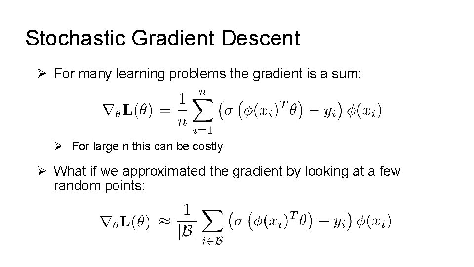
Stochastic Gradient Descent Ø For many learning problems the gradient is a sum: Ø For large n this can be costly Ø What if we approximated the gradient by looking at a few random points:

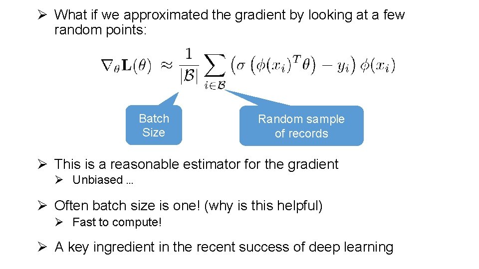
Ø What if we approximated the gradient by looking at a few random points: Batch Size Random sample of records Ø This is a reasonable estimator for the gradient Ø Unbiased … Ø Often batch size is one! (why is this helpful) Ø Fast to compute! Ø A key ingredient in the recent success of deep learning

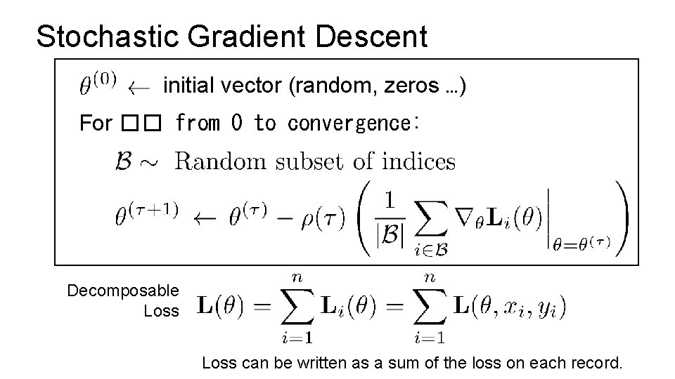
Stochastic Gradient Descent initial vector (random, zeros …) For �� from 0 to convergence: Decomposable Loss can be written as a sum of the loss on each record.

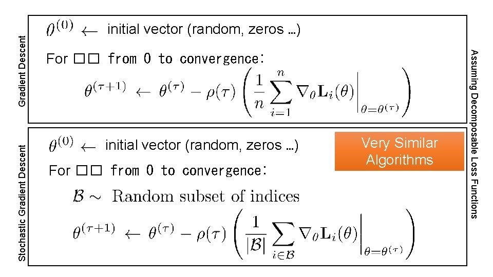
Gradient Descent For �� from 0 to convergence: initial vector (random, zeros …) For �� from 0 to convergence: Very Similar Algorithms Assuming Decomposable Loss Functions Stochastic Gradient Descent initial vector (random, zeros …)

Python Demo!

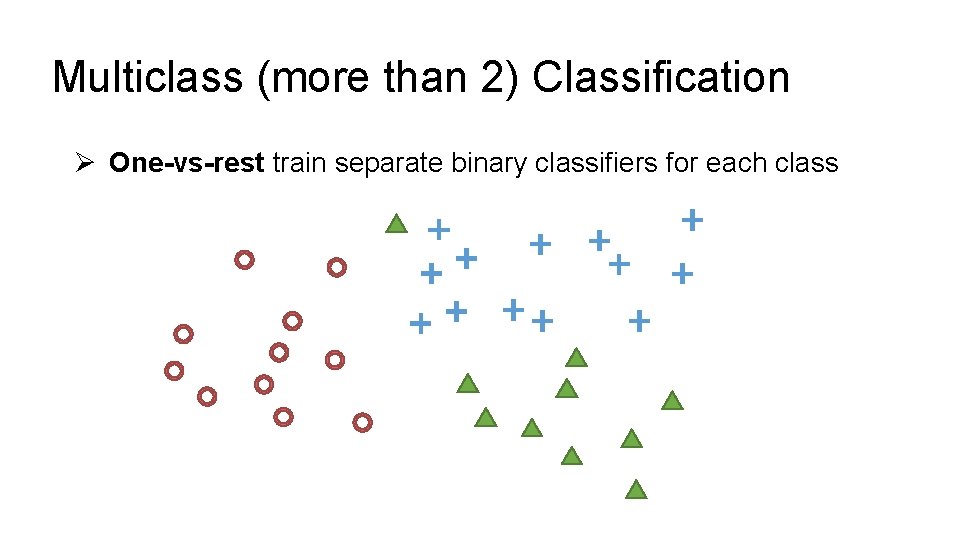
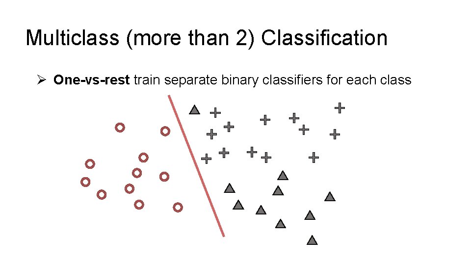
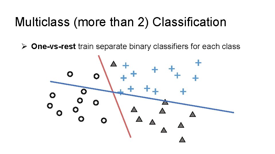
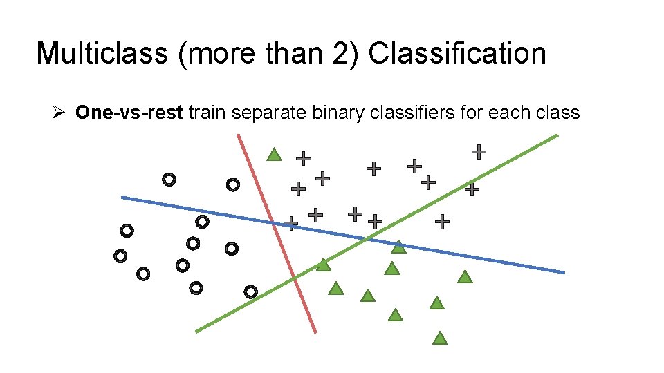
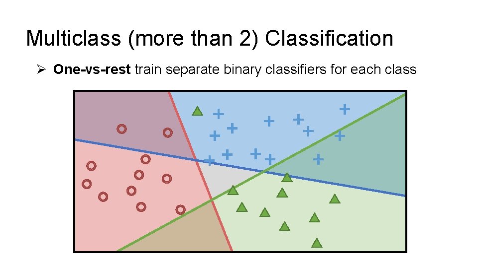
Multiclass (more than 2) Classification Ø One-vs-rest train separate binary classifiers for each class

Multiclass (more than 2) Classification Ø One-vs-rest train separate binary classifiers for each class

Multiclass (more than 2) Classification Ø One-vs-rest train separate binary classifiers for each class

Multiclass (more than 2) Classification Ø One-vs-rest train separate binary classifiers for each class

Multiclass (more than 2) Classification Ø One-vs-rest train separate binary classifiers for each class

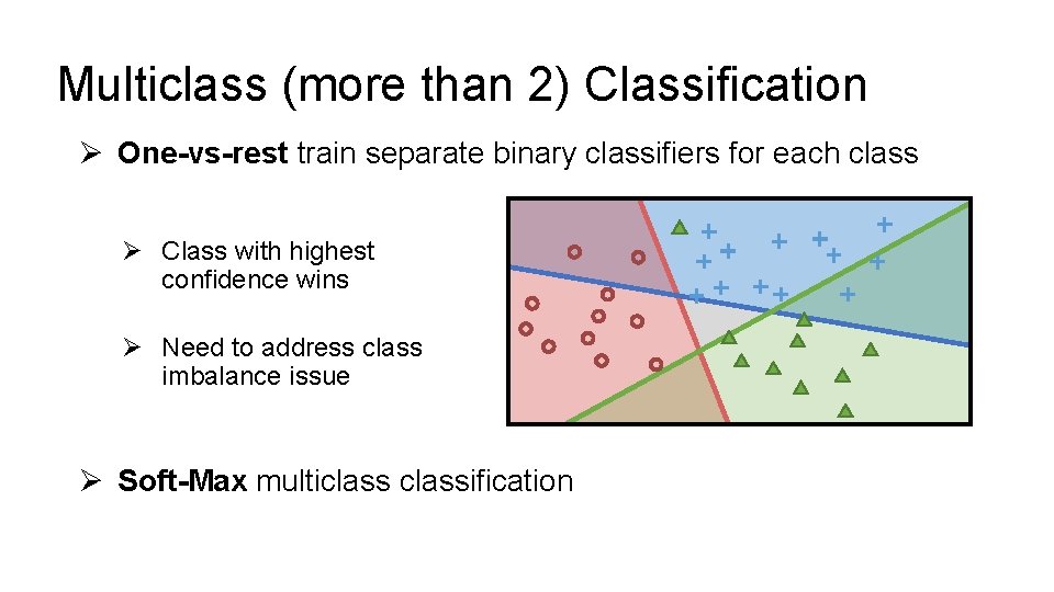
Multiclass (more than 2) Classification Ø One-vs-rest train separate binary classifiers for each class Ø Class with highest confidence wins Ø Need to address class imbalance issue Ø Soft-Max multiclassification

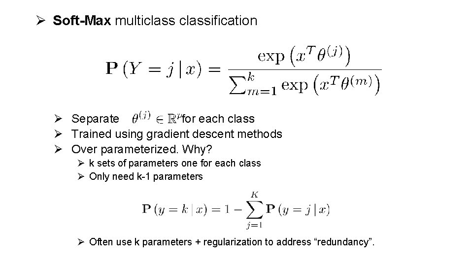
Ø Soft-Max multiclassification Ø Separate for each class Ø Trained using gradient descent methods Ø Over parameterized. Why? Ø k sets of parameters one for each class Ø Only need k-1 parameters Ø Often use k parameters + regularization to address “redundancy”.

Python Demo!

Deep Learning Overview Bonus Material Borrowed heavily from excellent talks by: • Adam Coates: http: //ai. stanford. edu/~acoates/coates_dltutorial_2013. pptx • Fei-Fei Li and Andrej Karpathy: http: //cs 231 n. stanford. edu/syllabus. html

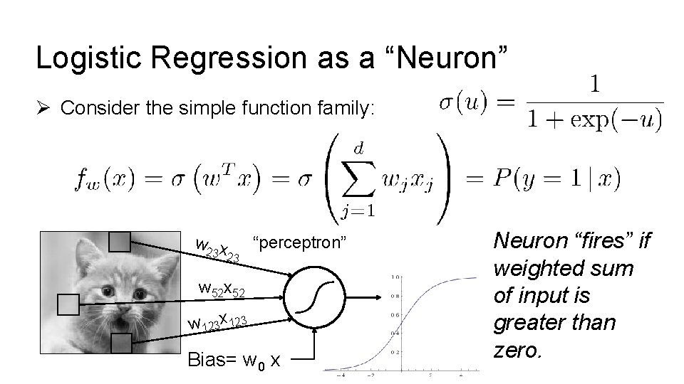
Logistic Regression as a “Neuron” Ø Consider the simple function family: w 2 x “perceptron” 3 23 w 52 x 52 w 123 x 123 Bias= w 0 x Neuron “fires” if weighted sum of input is greater than zero.

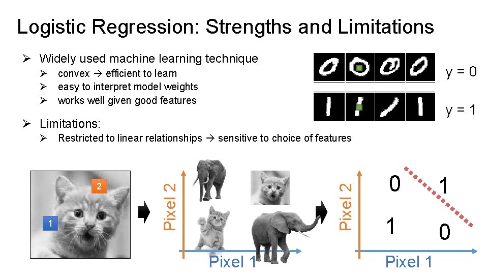
Logistic Regression: Strengths and Limitations Ø Widely used machine learning technique y=0 Ø convex efficient to learn Ø easy to interpret model weights Ø works well given good features y=1 Ø Limitations: 1 Pixel 2 2 Pixel 2 Ø Restricted to linear relationships sensitive to choice of features Pixel 1 0 1 1 0 Pixel 1

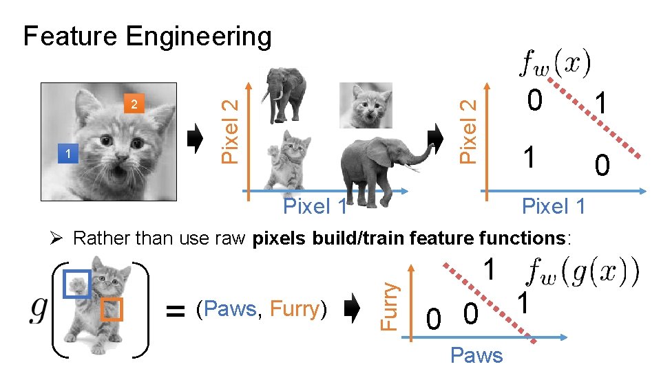
1 Pixel 2 2 Pixel 2 Feature Engineering Pixel 1 0 1 1 0 Pixel 1 = (Paws, Furry) Furry Ø Rather than use raw pixels build/train feature functions: 1 0 0 Paws 1

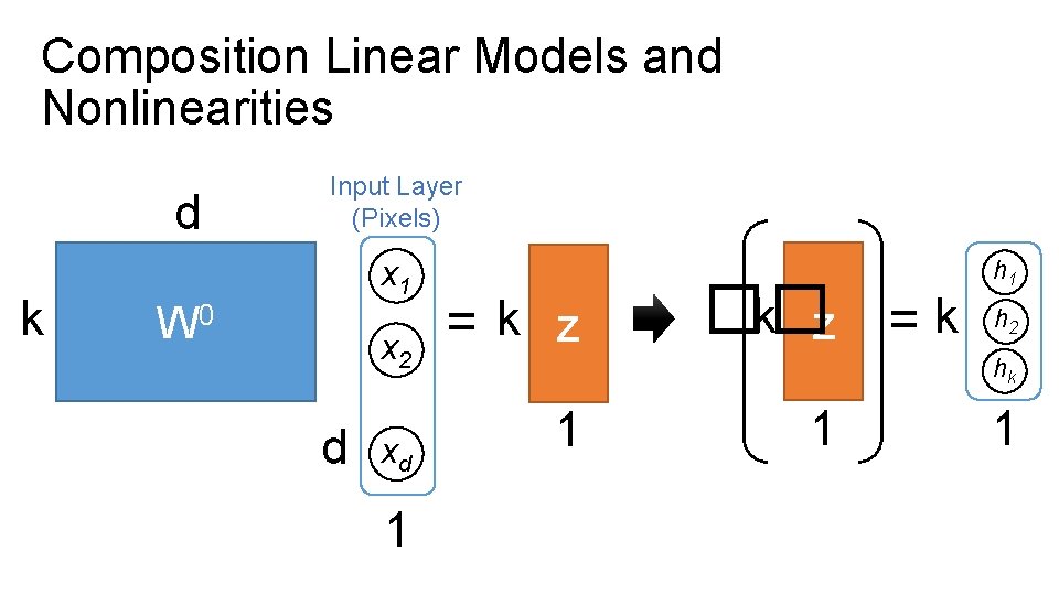
Composition Linear Models and Nonlinearities d k Input Layer (Pixels) x 1 W 0 x 2 d xd 1 =k z �� h 1 =k h 2 hk 1 1 1

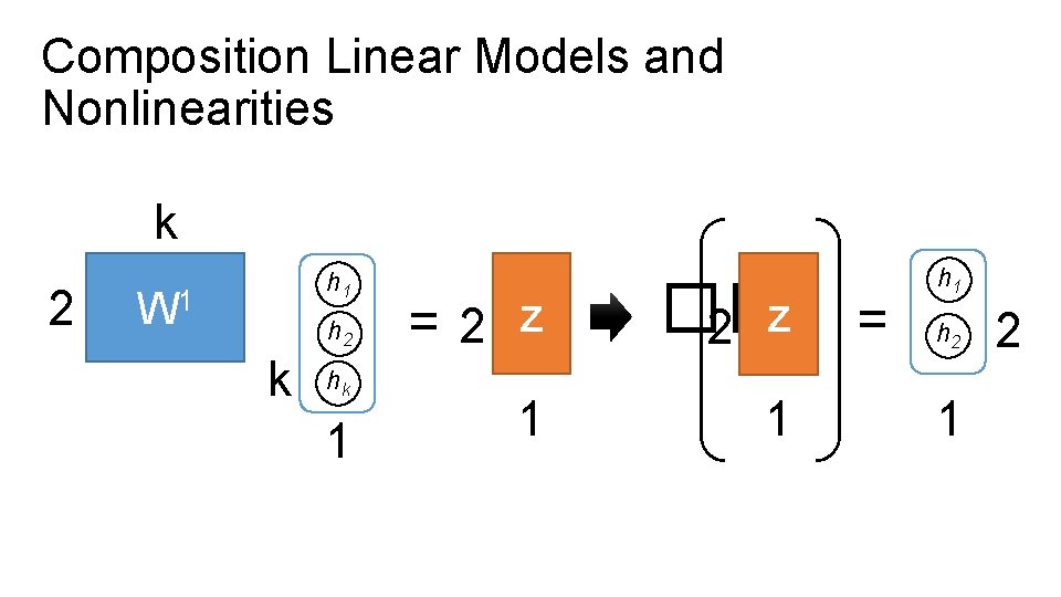
Composition Linear Models and Nonlinearities k 2 h 1 W 1 h 2 k hk 1 =2 z �� 2 z 1 1 = h 1 h 2 1 2

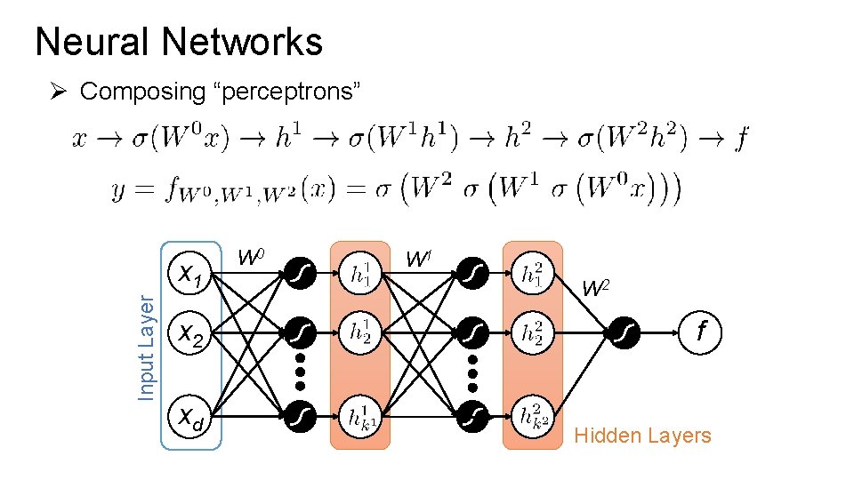
Neural Networks Ø Composing “perceptrons” Input Layer x 1 x 2 xd W 0 W 1 W 2 f Hidden Layers

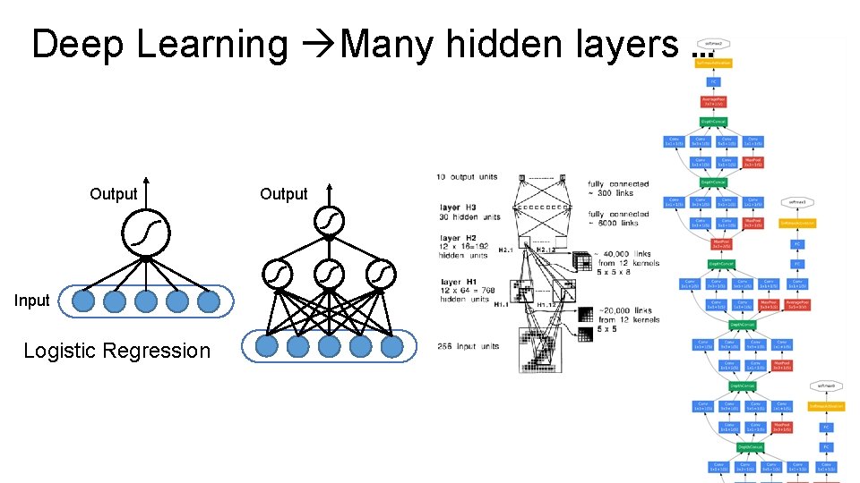
Deep Learning Many hidden layers … Output Input Logistic Regression Output

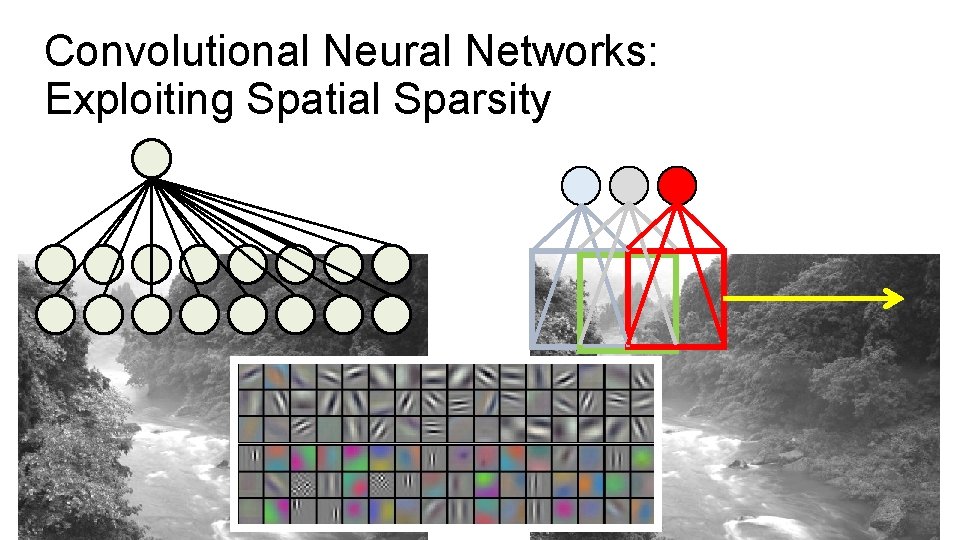
Convolutional Neural Networks: Exploiting Spatial Sparsity

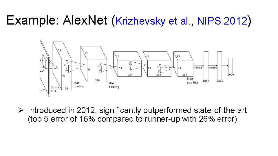
Example: Alex. Net (Krizhevsky et al. , NIPS 2012) Ø Introduced in 2012, significantly outperformed state-of-the-art (top 5 error of 16% compared to runner-up with 26% error)

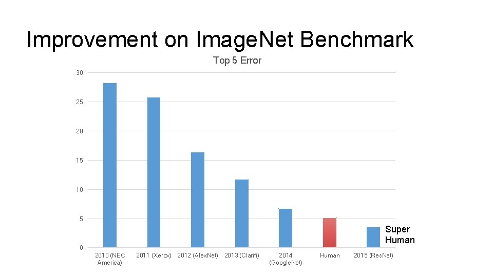
Improvement on Image. Net Benchmark Top 5 Error 30 25 20 15 10 5 Super Human 0 2010 (NEC America) 2011 (Xerox) 2012 (Alex. Net) 2013 (Clarifi) 2014 (Google. Net) Human 2015 (Res. Net)

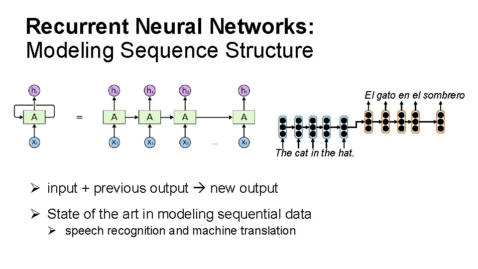
Recurrent Neural Networks: Modeling Sequence Structure El gato en el sombrero The cat in the hat. Ø input + previous output new output Ø State of the art in modeling sequential data Ø speech recognition and machine translation

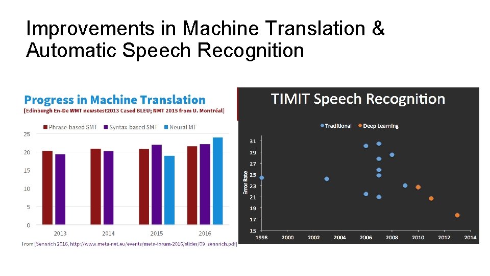
Improvements in Machine Translation & Automatic Speech Recognition

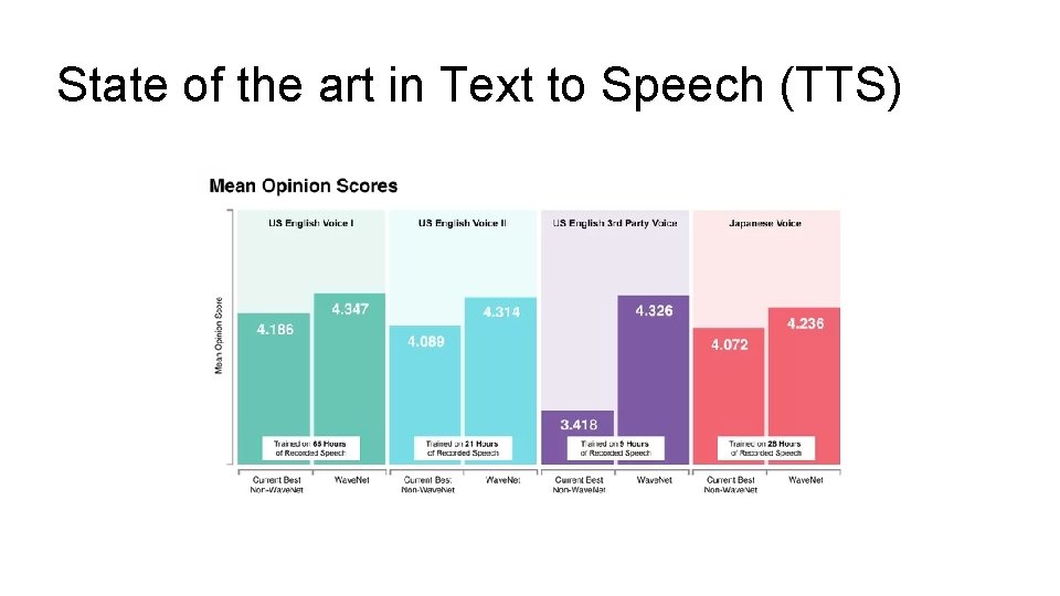
State of the art in Text to Speech (TTS)

Interested in Deep Learning? Ø RISE Lab Deep Learning Overview: Ø https: //ucbrise. github. io/cs 294 -rise-fa 16/deep_learning. html Ø Tensor. Flow Python Tutorial Ø Stanford CS 231 Labs Ø http: //cs 231 n. github. io/linear-classify/ Ø http: //cs 231 n. github. io/optimization-1/ Ø http: //cs 231 n. github. io/optimization-2/