Classification in Machine Learning Suchismit Mahapatra What is

Classification in Machine Learning Suchismit Mahapatra

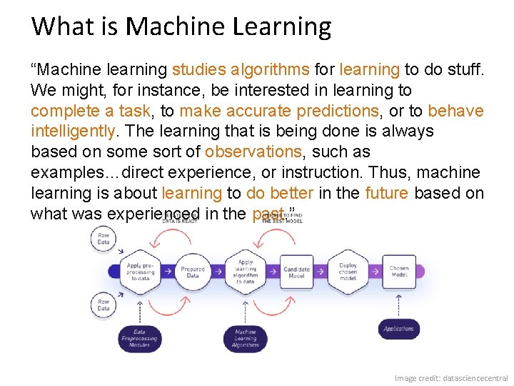
What is Machine Learning “Machine learning studies algorithms for learning to do stuff. We might, for instance, be interested in learning to complete a task, to make accurate predictions, or to behave intelligently. The learning that is being done is always based on some sort of observations, such as examples…direct experience, or instruction. Thus, machine learning is about learning to do better in the future based on what was experienced in the past. ” Image credit: datasciencecentral

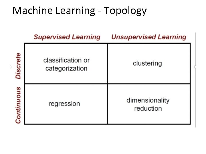
Machine Learning - Topology

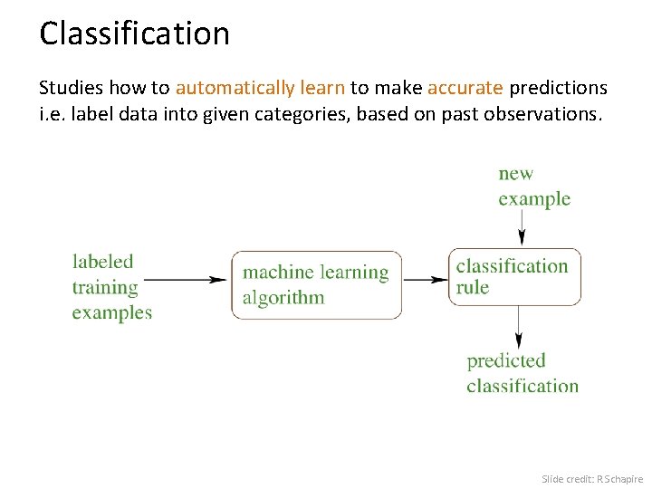
Classification Studies how to automatically learn to make accurate predictions i. e. label data into given categories, based on past observations. Slide credit: R. Schapire

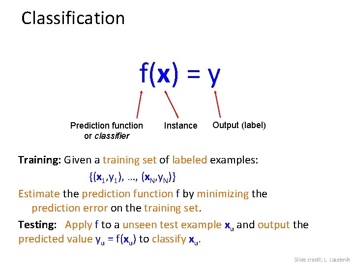
Classification f(x) = y Prediction function or classifier Instance Output (label) Training: Given a training set of labeled examples: {(x 1, y 1), …, (x. N, y. N)} Estimate the prediction function f by minimizing the prediction error on the training set. Testing: Apply f to a unseen test example xu and output the predicted value yu = f(xu) to classify xu. Slide credit: L. Lazebnik

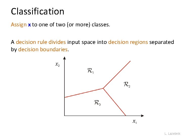
Classification Assign x to one of two (or more) classes. A decision rule divides input space into decision regions separated by decision boundaries. L. Lazebnik

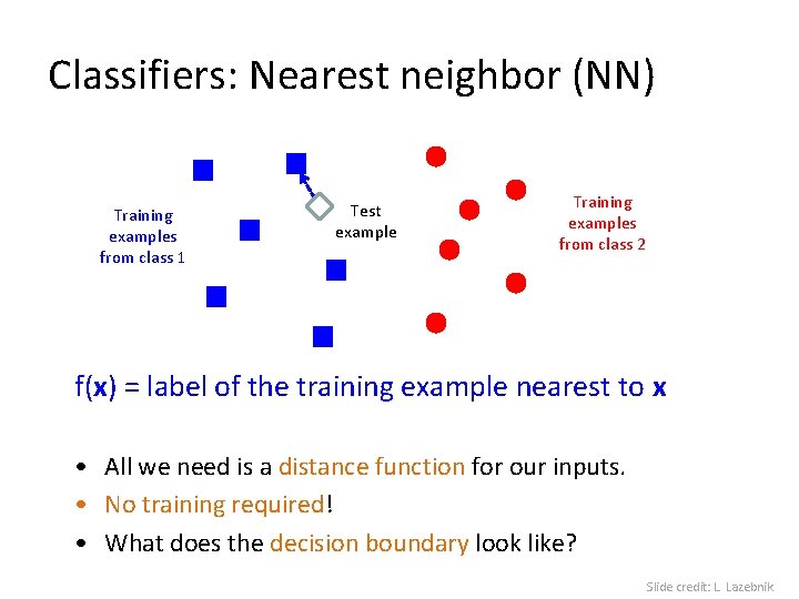
Classifiers: Nearest neighbor (NN) Training examples from class 1 Test example Training examples from class 2 f(x) = label of the training example nearest to x • All we need is a distance function for our inputs. • No training required! • What does the decision boundary look like? Slide credit: L. Lazebnik

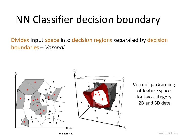
NN Classifier decision boundary Divides input space into decision regions separated by decision boundaries – Voronoi partitioning of feature space for two-category 2 D and 3 D data from Duda et al. Source: D. Lowe

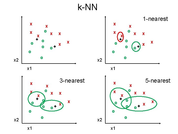
k-NN x x x 2 x o x + o o o x x o+ x x x 2 x 1 x x x 2 x o x + o o o x o+ x x 1 x o x + o o o x 1 1 -nearest x o+ 3 -nearest x x x 2 x o x + o o o x 1 5 -nearest x o+ x x x

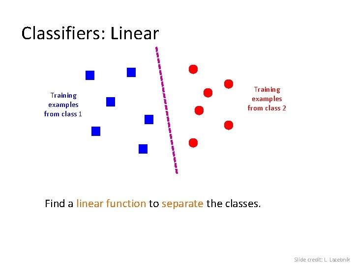
Classifiers: Linear Training examples from class 1 Training examples from class 2 Find a linear function to separate the classes. Slide credit: L. Lazebnik

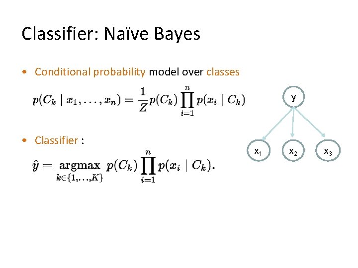
Classifier: Naïve Bayes • Conditional probability model over classes y • Classifier : x 1 x 2 x 3

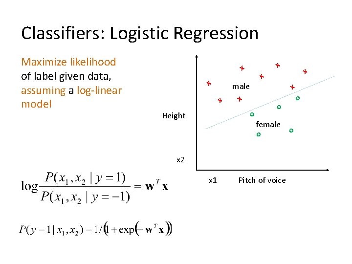
Classifiers: Logistic Regression Maximize likelihood of label given data, assuming a log-linear model x x male x x o Height o o female o x 2 x 1 x x Pitch of voice o

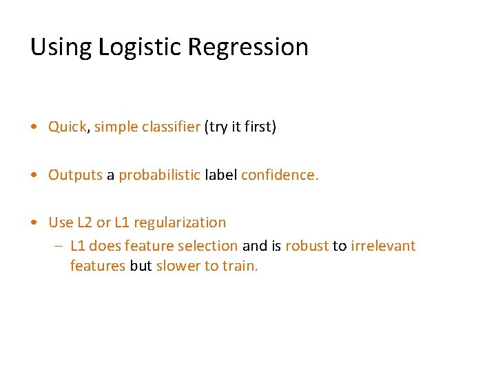
Using Logistic Regression • Quick, simple classifier (try it first) • Outputs a probabilistic label confidence. • Use L 2 or L 1 regularization – L 1 does feature selection and is robust to irrelevant features but slower to train.

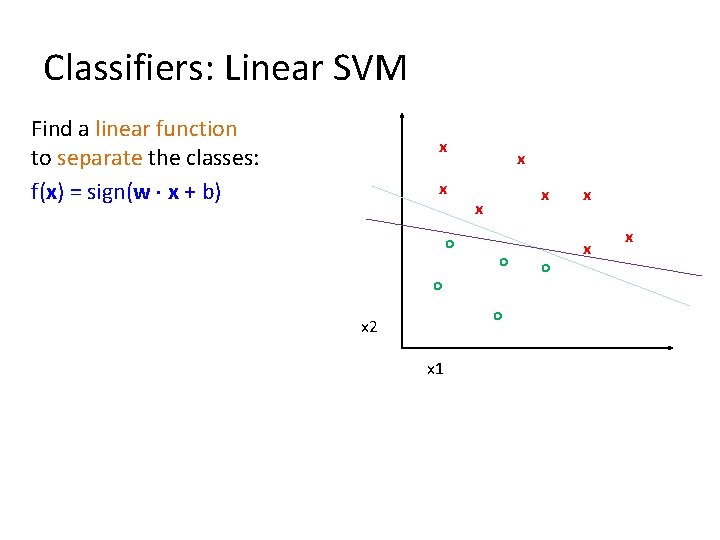
Classifiers: Linear SVM Find a linear function to separate the classes: f(x) = sign(w x + b) x x o x x x o o o x 2 x 1 o x x x

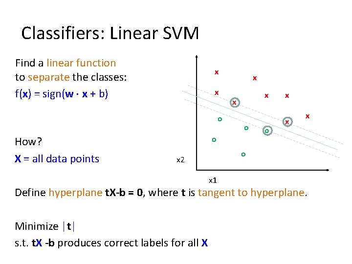
Classifiers: Linear SVM Find a linear function to separate the classes: f(x) = sign(w x + b) x x o How? X = all data points x x x o o o x x x o x 2 x 1 Define hyperplane t. X-b = 0, where t is tangent to hyperplane. Minimize |t| s. t. t. X -b produces correct labels for all X

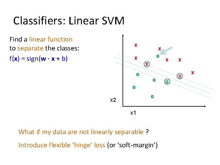
Classifiers: Linear SVM Find a linear function to separate the classes: f(x) = sign(w x + b) x x x o o o o x 2 x 1 What if my data are not linearly separable ? Introduce flexible ‘hinge’ loss (or ‘soft-margin’) x o x x x

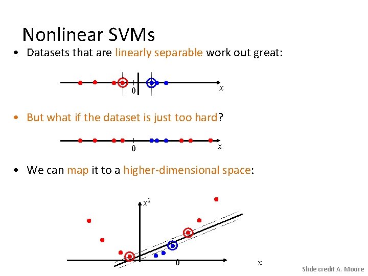
Nonlinear SVMs • Datasets that are linearly separable work out great: x 0 • But what if the dataset is just too hard? x 0 • We can map it to a higher-dimensional space: x 2 0 x Slide credit A. Moore

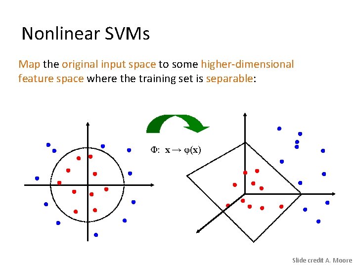
Nonlinear SVMs Map the original input space to some higher-dimensional feature space where the training set is separable: Φ: x → φ(x) Slide credit A. Moore

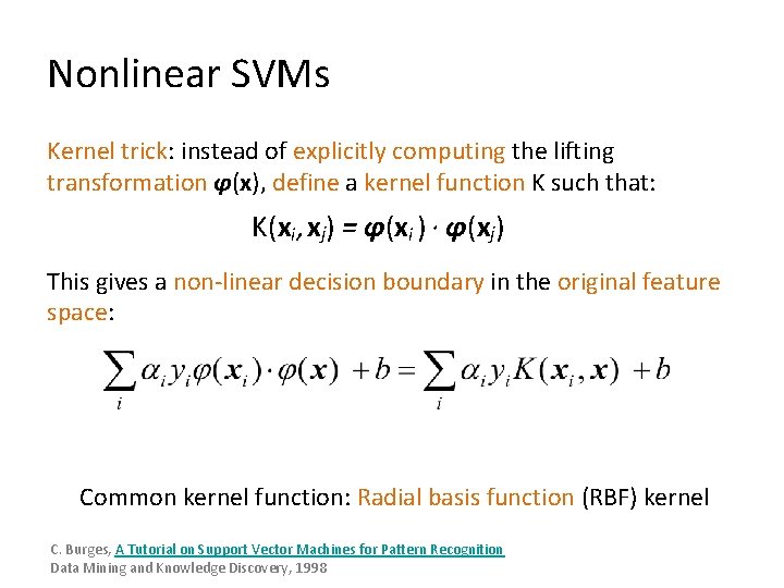
Nonlinear SVMs Kernel trick: instead of explicitly computing the lifting transformation φ(x), define a kernel function K such that: K(xi , xj) = φ(xi ) · φ(xj) This gives a non-linear decision boundary in the original feature space: Common kernel function: Radial basis function (RBF) kernel C. Burges, A Tutorial on Support Vector Machines for Pattern Recognition Data Mining and Knowledge Discovery, 1998

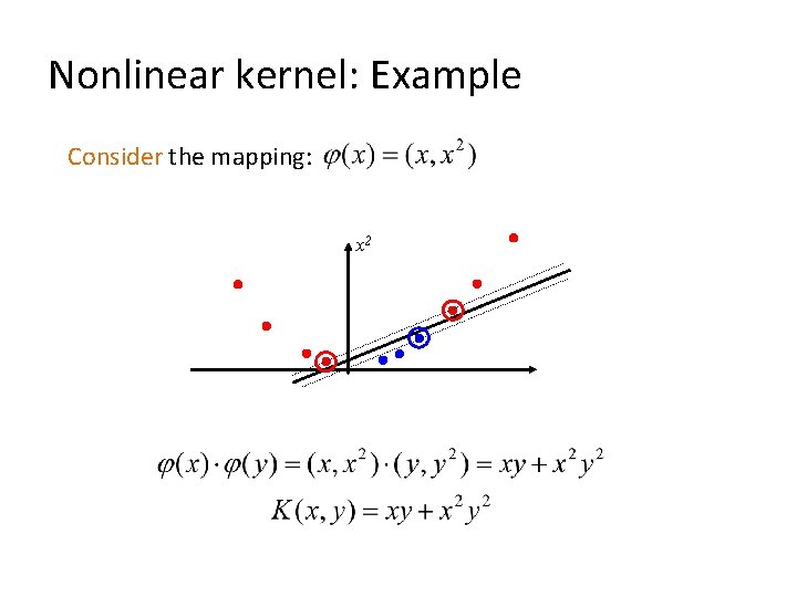
Nonlinear kernel: Example Consider the mapping: x 2

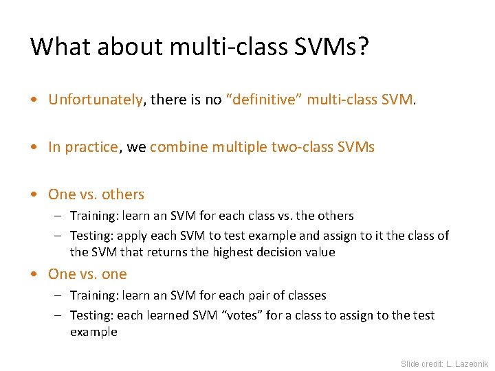
What about multi-class SVMs? • Unfortunately, there is no “definitive” multi-class SVM. • In practice, we combine multiple two-class SVMs • One vs. others – Training: learn an SVM for each class vs. the others – Testing: apply each SVM to test example and assign to it the class of the SVM that returns the highest decision value • One vs. one – Training: learn an SVM for each pair of classes – Testing: each learned SVM “votes” for a class to assign to the test example Slide credit: L. Lazebnik

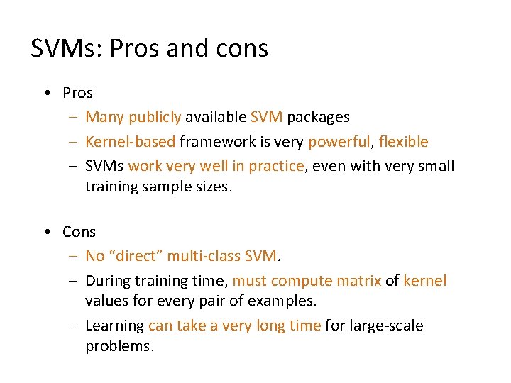
SVMs: Pros and cons • Pros – Many publicly available SVM packages – Kernel-based framework is very powerful, flexible – SVMs work very well in practice, even with very small training sample sizes. • Cons – No “direct” multi-class SVM. – During training time, must compute matrix of kernel values for every pair of examples. – Learning can take a very long time for large-scale problems.

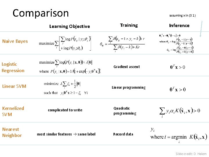
Comparison Learning Objective assuming x in {0 1} Training Inference Naïve Bayes Logistic Regression Gradient ascent Linear SVM Kernelized SVM Nearest Neighbor Linear programming complicated to write most similar features same label Quadratic programming Record data Slide credit: D. Hoiem

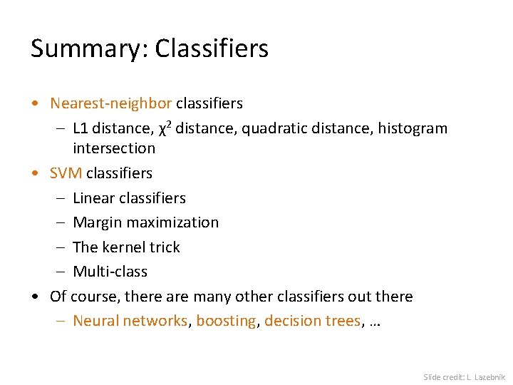
Summary: Classifiers • Nearest-neighbor classifiers – L 1 distance, χ2 distance, quadratic distance, histogram intersection • SVM classifiers – Linear classifiers – Margin maximization – The kernel trick – Multi-class • Of course, there are many other classifiers out there – Neural networks, boosting, decision trees, … Slide credit: L. Lazebnik

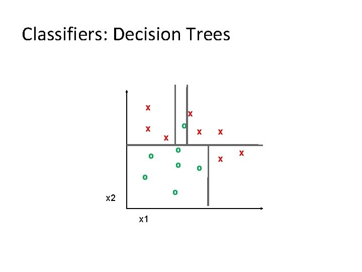
Classifiers: Decision Trees x x o x o o x 2 x 1 x o x x x

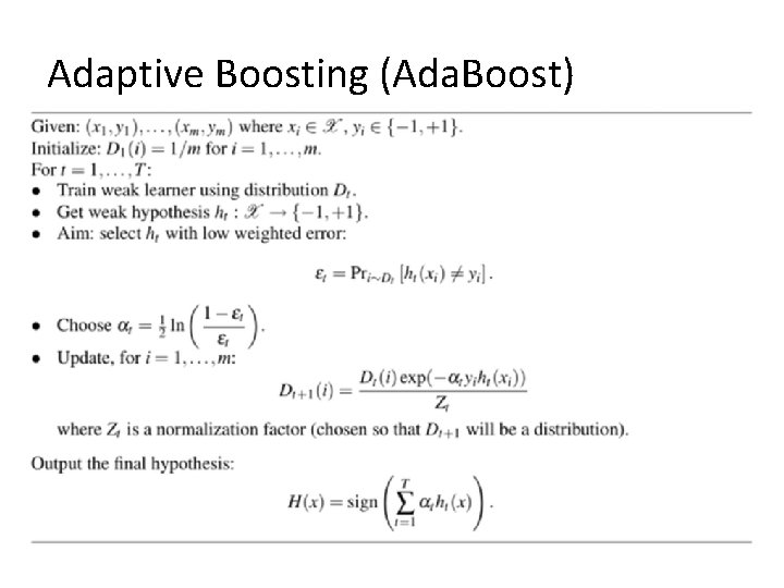
Adaptive Boosting (Ada. Boost)

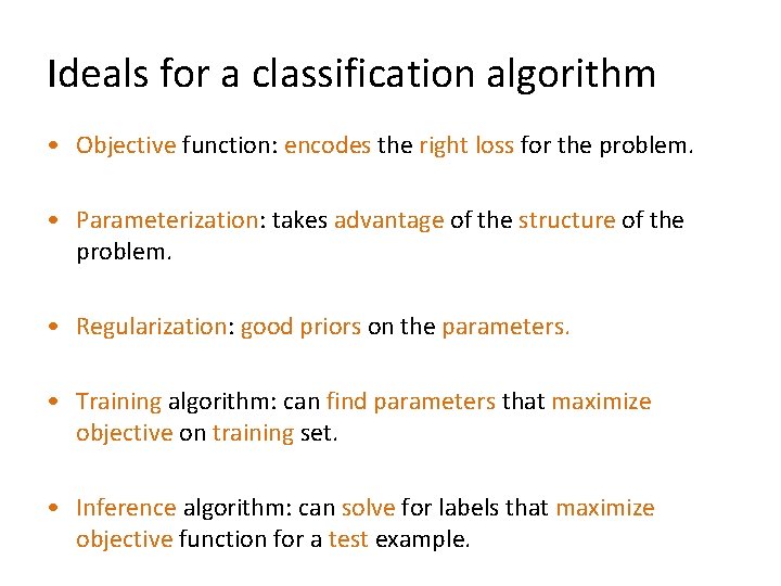
Ideals for a classification algorithm • Objective function: encodes the right loss for the problem. • Parameterization: takes advantage of the structure of the problem. • Regularization: good priors on the parameters. • Training algorithm: can find parameters that maximize objective on training set. • Inference algorithm: can solve for labels that maximize objective function for a test example.

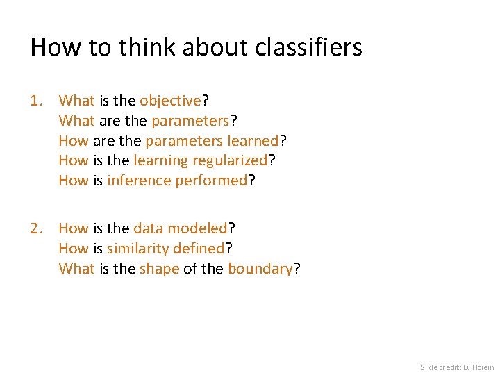
How to think about classifiers 1. What is the objective? What are the parameters? How are the parameters learned? How is the learning regularized? How is inference performed? 2. How is the data modeled? How is similarity defined? What is the shape of the boundary? Slide credit: D. Hoiem

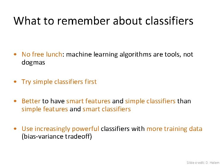
What to remember about classifiers • No free lunch: machine learning algorithms are tools, not dogmas • Try simple classifiers first • Better to have smart features and simple classifiers than simple features and smart classifiers • Use increasingly powerful classifiers with more training data (bias-variance tradeoff) Slide credit: D. Hoiem

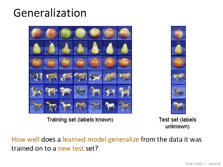
Generalization Training set (labels known) Test set (labels unknown) How well does a learned model generalize from the data it was trained on to a new test set? Slide credit: L. Lazebnik

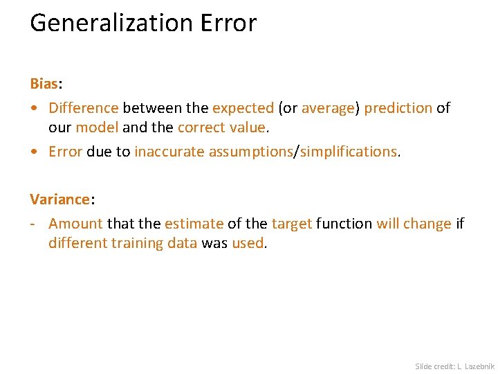
Generalization Error Bias: • Difference between the expected (or average) prediction of our model and the correct value. • Error due to inaccurate assumptions/simplifications. Variance: - Amount that the estimate of the target function will change if different training data was used. Slide credit: L. Lazebnik

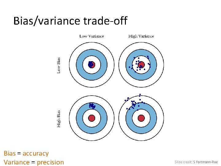
Bias/variance trade-off Bias = accuracy Variance = precision Slide credit: S Fortmann-Roe

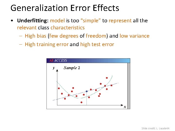
Generalization Error Effects • Underfitting: model is too “simple” to represent all the relevant class characteristics – High bias (few degrees of freedom) and low variance – High training error and high test error Slide credit: L. Lazebnik

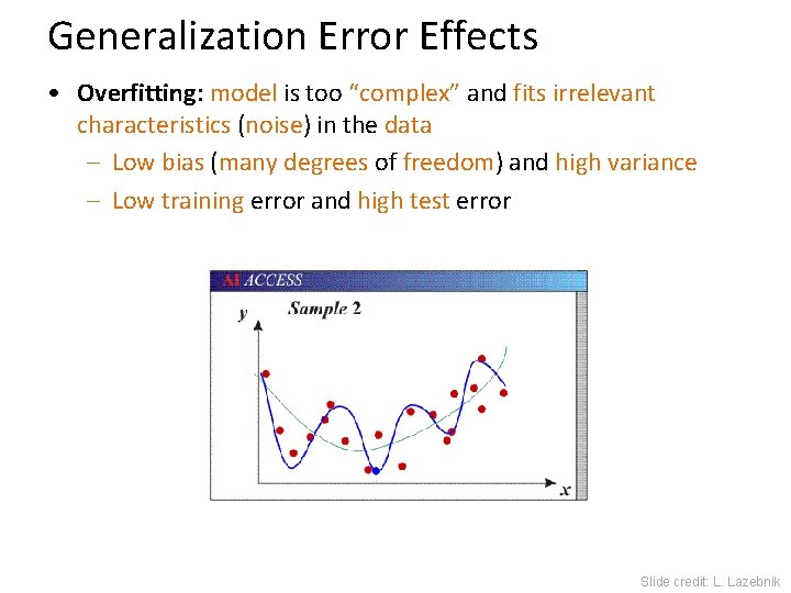
Generalization Error Effects • Overfitting: model is too “complex” and fits irrelevant characteristics (noise) in the data – Low bias (many degrees of freedom) and high variance – Low training error and high test error Slide credit: L. Lazebnik

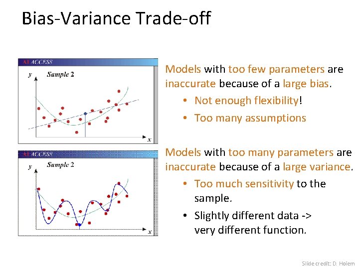
Bias-Variance Trade-off Models with too few parameters are inaccurate because of a large bias. • Not enough flexibility! • Too many assumptions Models with too many parameters are inaccurate because of a large variance. • Too much sensitivity to the sample. • Slightly different data -> very different function. Slide credit: D. Hoiem

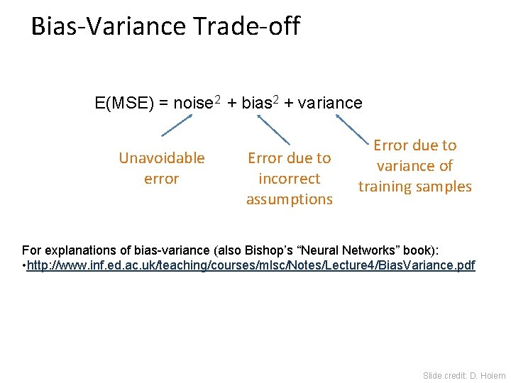
Bias-Variance Trade-off E(MSE) = noise 2 + bias 2 + variance Unavoidable error Error due to incorrect assumptions Error due to variance of training samples For explanations of bias-variance (also Bishop’s “Neural Networks” book): • http: //www. inf. ed. ac. uk/teaching/courses/mlsc/Notes/Lecture 4/Bias. Variance. pdf Slide credit: D. Hoiem

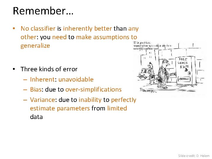
Remember… • No classifier is inherently better than any other: you need to make assumptions to generalize • Three kinds of error – Inherent: unavoidable – Bias: due to over-simplifications – Variance: due to inability to perfectly estimate parameters from limited data Slide credit: D. Hoiem

How to reduce variance? • Choose a simpler classifier • Regularize the parameters • Get more training data Slide credit: D. Hoiem

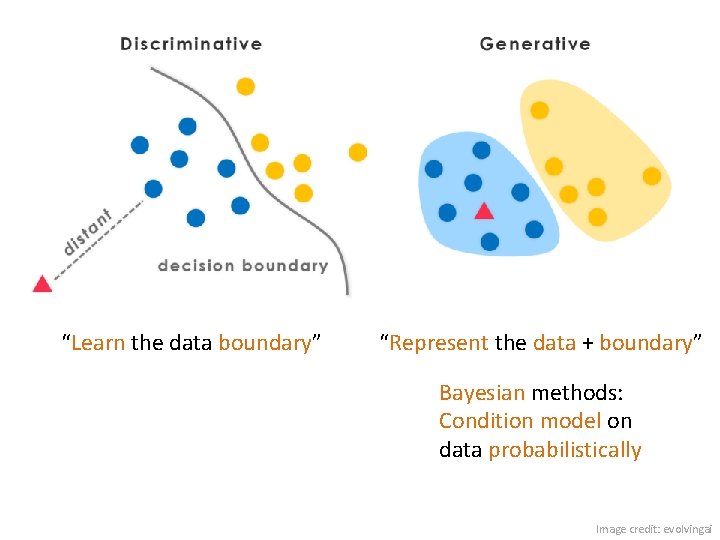
“Learn the data boundary” “Represent the data + boundary” Bayesian methods: Condition model on data probabilistically Image credit: evolvingai

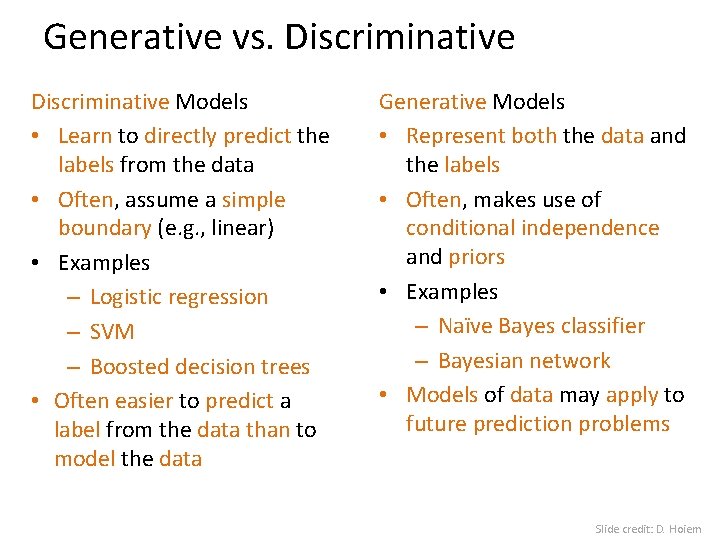
Generative vs. Discriminative Models • Learn to directly predict the labels from the data • Often, assume a simple boundary (e. g. , linear) • Examples – Logistic regression – SVM – Boosted decision trees • Often easier to predict a label from the data than to model the data Generative Models • Represent both the data and the labels • Often, makes use of conditional independence and priors • Examples – Naïve Bayes classifier – Bayesian network • Models of data may apply to future prediction problems Slide credit: D. Hoiem

Making decisions about data • Important design decisions: 1) What data do I use? 2) How do I represent my data ? 3) What classifier / regressor do I use? • These are in decreasing order of importance • Deep learning addresses 2 and 3 simultaneously (and blurs the boundary between them). • You can take the representation from deep learning and use it with any classifier.

Many classifiers to choose from… • • • K-nearest neighbor SVM Naïve Bayesian network Which Logistic regression Randomized Forests Boosted Decision Trees Restricted Boltzmann Machines Neural networks … is the best?