Classification Giuseppe Attardi Universit di Pisa Classification l

Classification Giuseppe Attardi Università di Pisa

Classification l Define classes/categories l Label text l Extract features l Choose a classifier § Naive Bayes Classifier § Decision Trees § Maximum Entropy § … l Train it l Use it to classify new examples

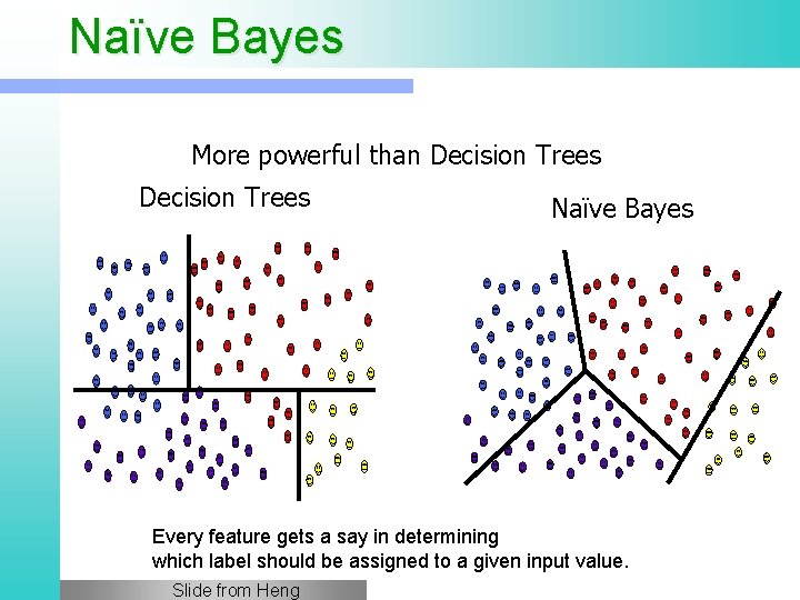
Naïve Bayes More powerful than Decision Trees Naïve Bayes Every feature gets a say in determining which label should be assigned to a given input value. Slide from Heng

Naïve Bayes: Strengths l l l Very simple model § Easy to understand § Very easy to implement Can scale easily to millions of training examples (just need counts!) Very efficient, fast training and classification Modest space storage Widely used because it works really well for text categorization Linear, but non parallel decision boundaries Slide from Heng

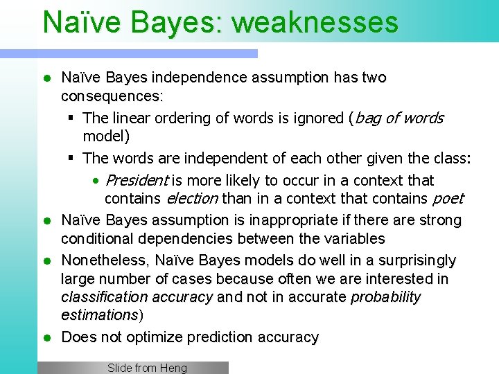
Naïve Bayes: weaknesses Naïve Bayes independence assumption has two consequences: § The linear ordering of words is ignored (bag of words model) § The words are independent of each other given the class: • President is more likely to occur in a context that contains election than in a context that contains poet l Naïve Bayes assumption is inappropriate if there are strong conditional dependencies between the variables l Nonetheless, Naïve Bayes models do well in a surprisingly large number of cases because often we are interested in classification accuracy and not in accurate probability estimations) l Does not optimize prediction accuracy l Slide from Heng

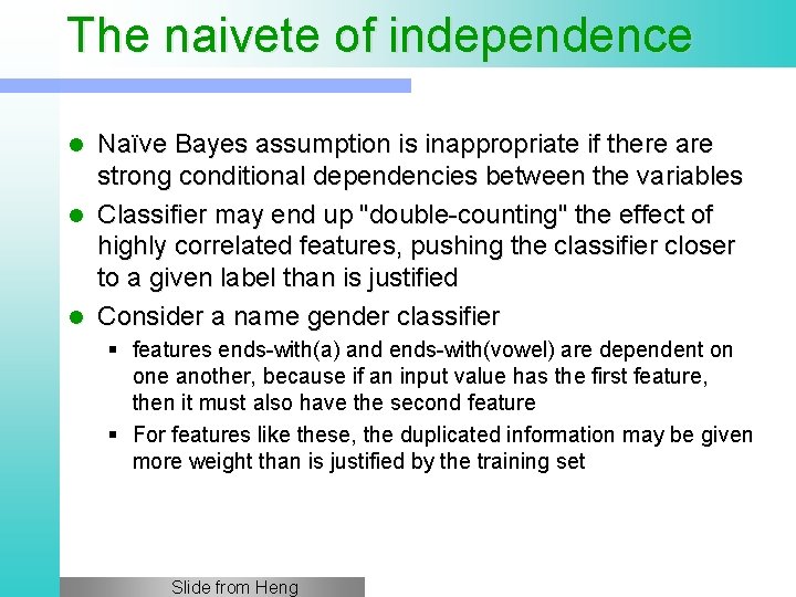
The naivete of independence Naïve Bayes assumption is inappropriate if there are strong conditional dependencies between the variables l Classifier may end up "double-counting" the effect of highly correlated features, pushing the classifier closer to a given label than is justified l Consider a name gender classifier l § features ends-with(a) and ends-with(vowel) are dependent on one another, because if an input value has the first feature, then it must also have the second feature § For features like these, the duplicated information may be given more weight than is justified by the training set Slide from Heng

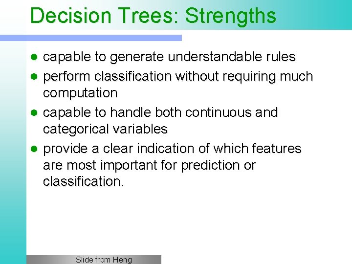
Decision Trees: Strengths l l capable to generate understandable rules perform classification without requiring much computation capable to handle both continuous and categorical variables provide a clear indication of which features are most important for prediction or classification. Slide from Heng

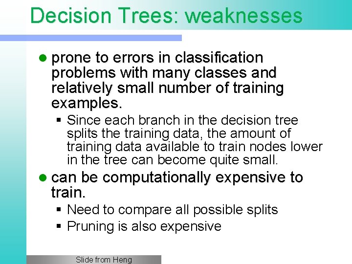
Decision Trees: weaknesses l prone to errors in classification problems with many classes and relatively small number of training examples. § Since each branch in the decision tree splits the training data, the amount of training data available to train nodes lower in the tree can become quite small. l can be computationally expensive to train. § Need to compare all possible splits § Pruning is also expensive Slide from Heng

Decision Trees: weaknesses Typically examine one field at a time l Leads to rectangular classification boxes that may not correspond well with the actual distribution of records in the decision space. § Such ordering limits their ability to exploit features that are relatively independent of one another § Naive Bayes overcomes this limitation by allowing all features to act "in parallel" l Slide from Heng

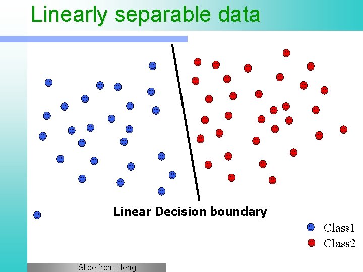
Linearly separable data Linear Decision boundary Class 1 Class 2 Slide from Heng

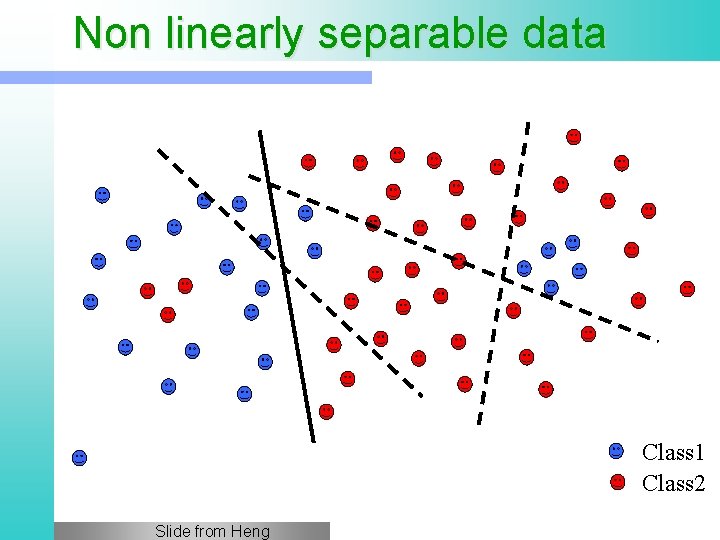
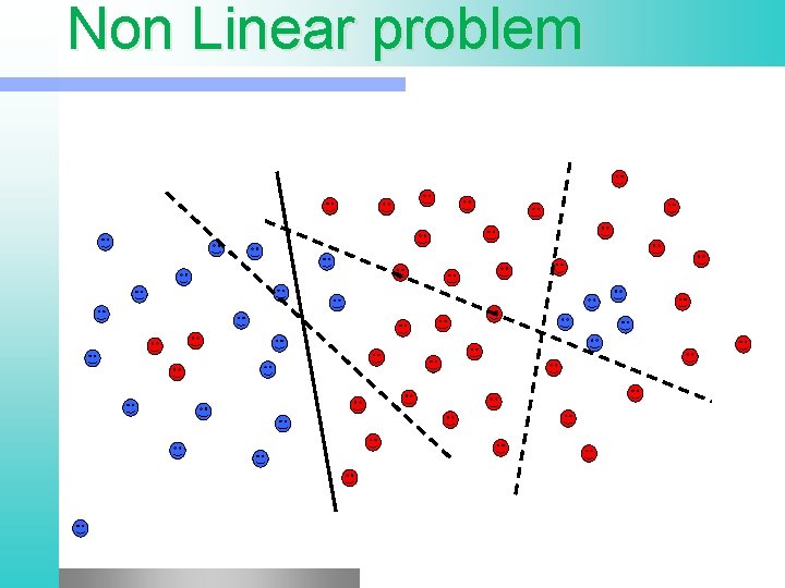
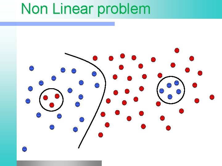
Non linearly separable data Class 1 Class 2 Slide from Heng

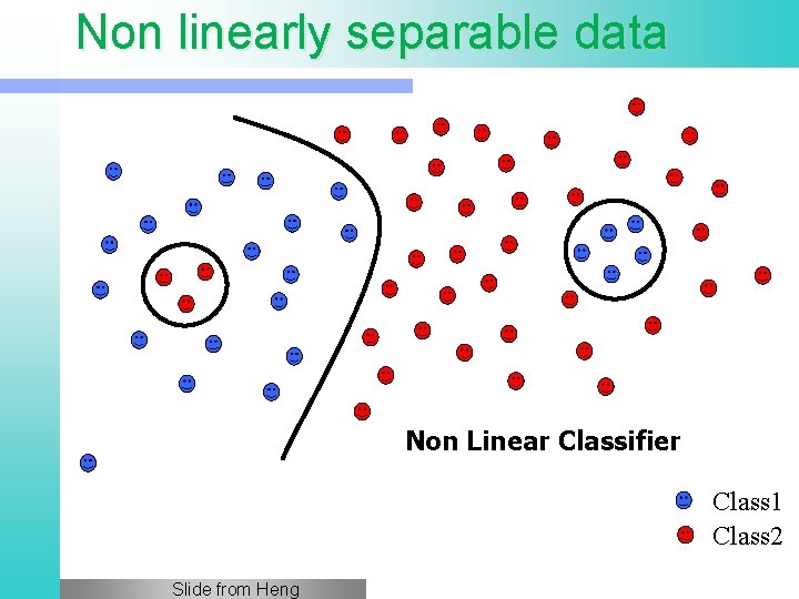
Non linearly separable data Non Linear Classifier Class 1 Class 2 Slide from Heng

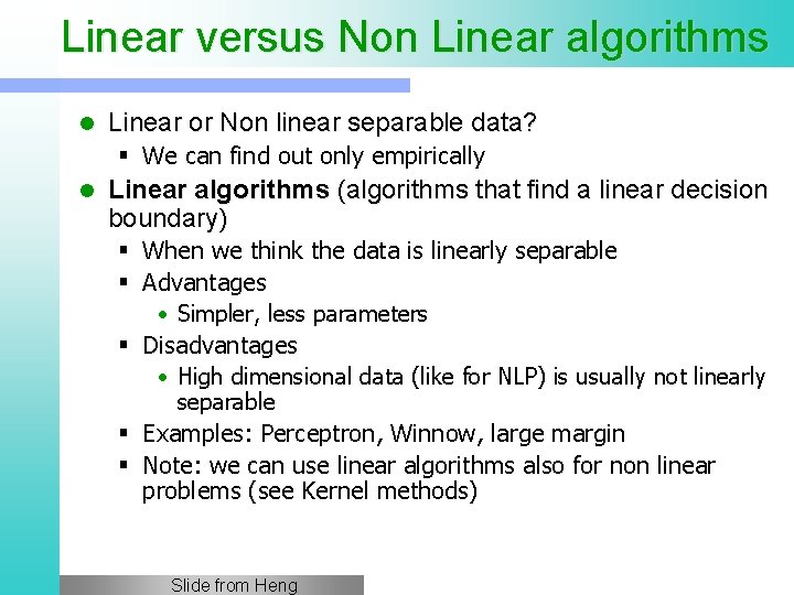
Linear versus Non Linear algorithms l Linear or Non linear separable data? § We can find out only empirically l Linear algorithms (algorithms that find a linear decision boundary) § When we think the data is linearly separable § Advantages • Simpler, less parameters § Disadvantages • High dimensional data (like for NLP) is usually not linearly separable § Examples: Perceptron, Winnow, large margin § Note: we can use linear algorithms also for non linear problems (see Kernel methods) Slide from Heng

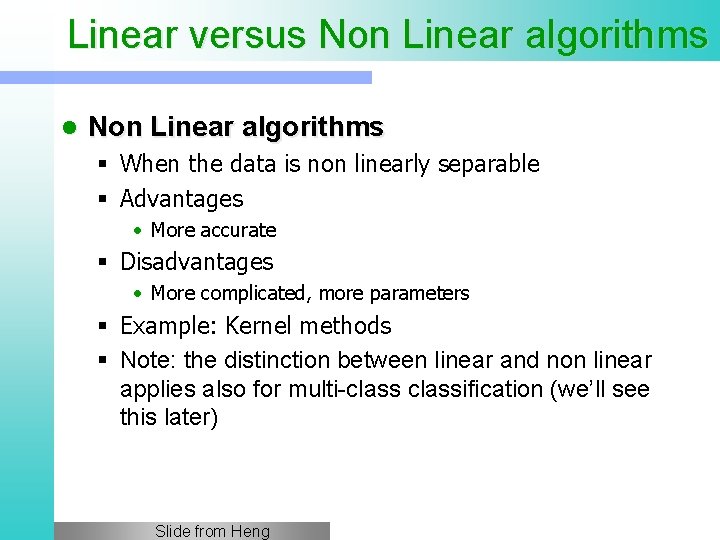
Linear versus Non Linear algorithms l Non Linear algorithms § When the data is non linearly separable § Advantages • More accurate § Disadvantages • More complicated, more parameters § Example: Kernel methods § Note: the distinction between linear and non linear applies also for multi-classification (we’ll see this later) Slide from Heng

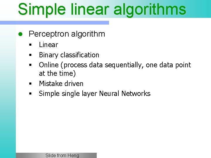
Simple linear algorithms l Perceptron algorithm § Linear § Binary classification § Online (process data sequentially, one data point at the time) § Mistake driven § Simple single layer Neural Networks Slide from Heng

Linear Algebra

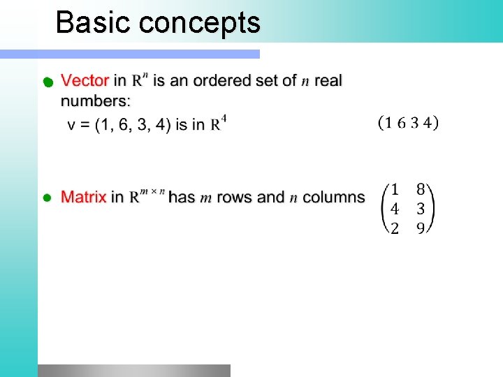
Basic concepts l

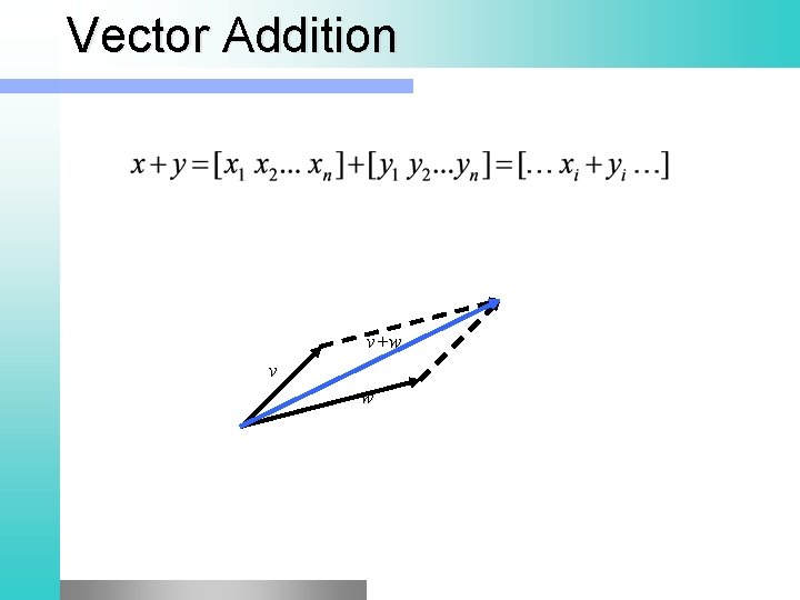
Vector Addition v+w v w

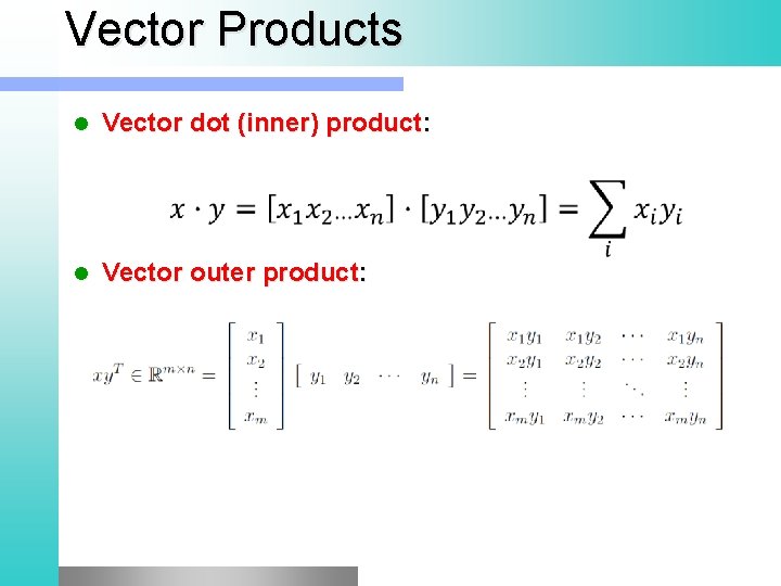
Vector Products l Vector dot (inner) product: l Vector outer product:

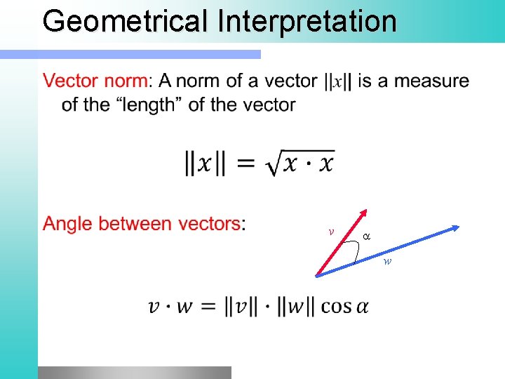
Geometrical Interpretation v w

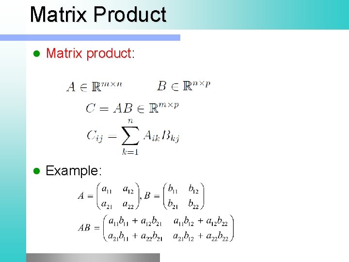
Matrix Product l Matrix product: l Example:

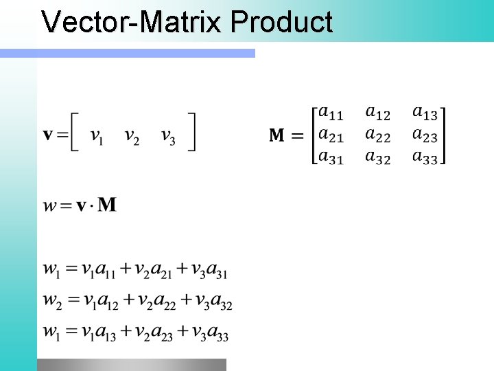
Vector-Matrix Product

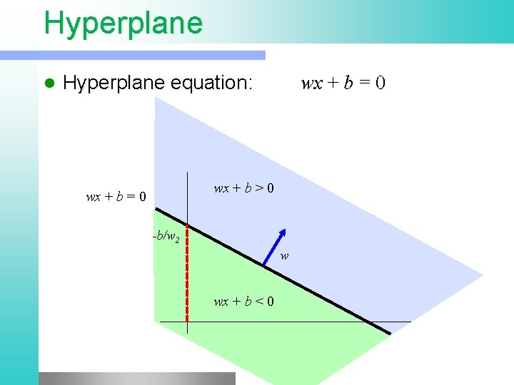
Hyperplane l Hyperplane equation: wx + b = 0 wx + b > 0 wx + b = 0 -b/w 2 w wx + b < 0

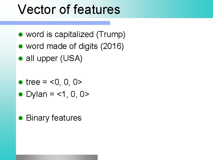
Vector of features word is capitalized (Trump) l word made of digits (2016) l all upper (USA) l tree = <0, 0, 0> l Dylan = <1, 0, 0> l l Binary features

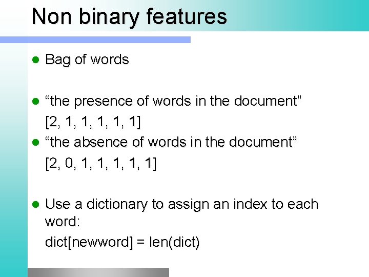
Non binary features l Bag of words “the presence of words in the document” [2, 1, 1, 1] l “the absence of words in the document” [2, 0, 1, 1, 1] l l Use a dictionary to assign an index to each word: dict[newword] = len(dict)

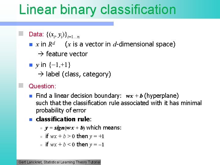
Linear binary classification n Data: {(xi, yi)}i=1…n n n x in Rd (x is a vector in d-dimensional space) feature vector y in { 1, +1} label (class, category) n Question: n n Find a linear decision boundary: wx + b (hyperplane) such that the classification rule associated with it has minimal probability of error classification rule: n n n y = sign(w x + b) which means: if wx + b > 0 then y = +1 if wx + b < 0 then y = 1 Gert Lanckriet, Statistical Learning Theory Tutorial

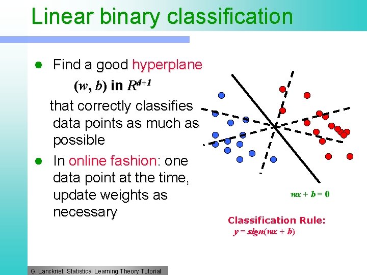
Linear binary classification Find a good hyperplane (w, b) in Rd+1 that correctly classifies data points as much as possible l In online fashion: one data point at the time, update weights as necessary l G. Lanckriet, Statistical Learning Theory Tutorial wx + b = 0 Classification Rule: y = sign(wx + b)

Perceptron

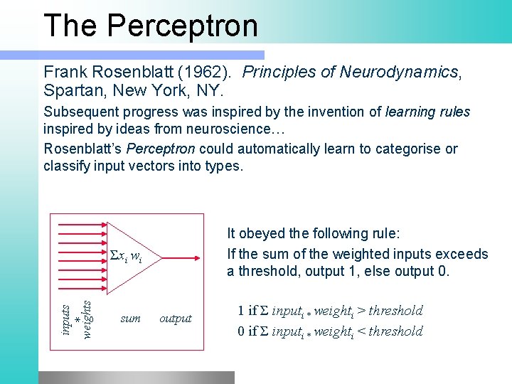
The Perceptron Frank Rosenblatt (1962). Principles of Neurodynamics, Spartan, New York, NY. Subsequent progress was inspired by the invention of learning rules inspired by ideas from neuroscience… Rosenblatt’s Perceptron could automatically learn to categorise or classify input vectors into types. It obeyed the following rule: If the sum of the weighted inputs exceeds a threshold, output 1, else output 0. inputs * weights Σxi wi sum output 1 if Σ inputi * weighti > threshold 0 if Σ inputi * weighti < threshold

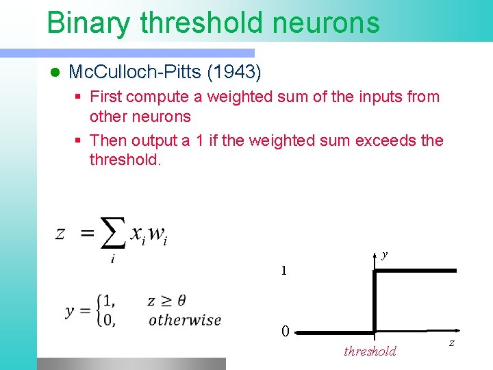
Binary threshold neurons l Mc. Culloch-Pitts (1943) § First compute a weighted sum of the inputs from other neurons § Then output a 1 if the weighted sum exceeds the threshold. y 1 0 threshold z

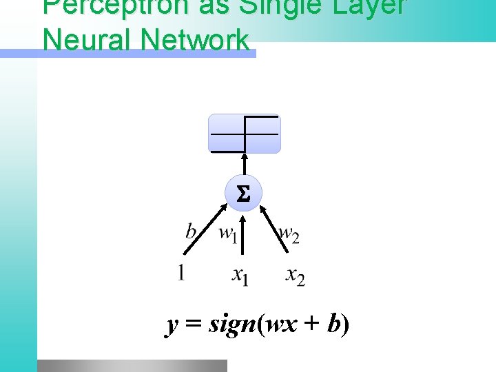
Perceptron as Single Layer Neural Network S y = sign(wx + b)

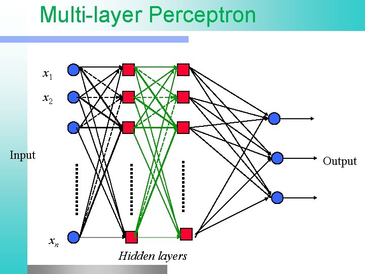
Multi-layer Perceptron x 1 x 2 Input Output xn Hidden layers

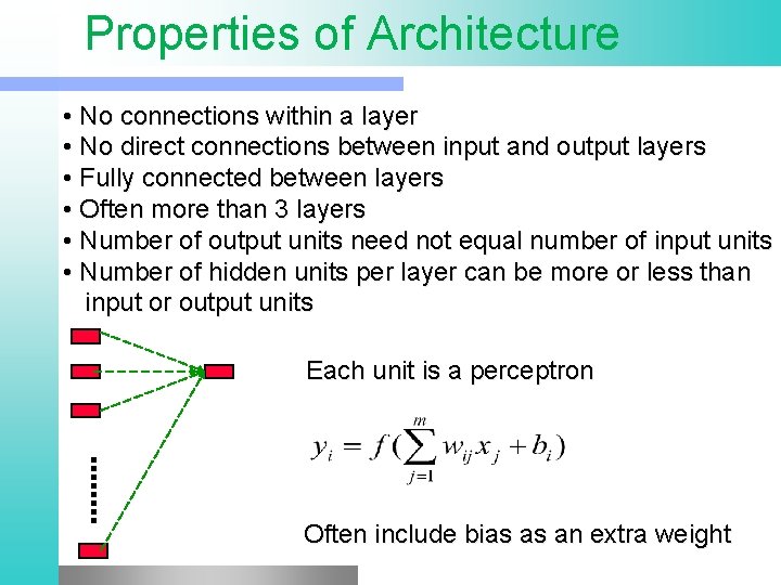
Properties of Architecture • No connections within a layer • No direct connections between input and output layers • Fully connected between layers • Often more than 3 layers • Number of output units need not equal number of input units • Number of hidden units per layer can be more or less than input or output units Each unit is a perceptron Often include bias as an extra weight

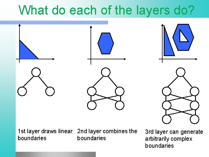
What do each of the layers do? 1 st layer draws linear 2 nd layer combines the boundaries 3 rd layer can generate arbitrarily complex boundaries

Perceptron Learning Rule Assuming the problem is linearly separable, there is a learning rule that converges in a finite time Motivation A new (unseen) input pattern that is similar to an old (seen) input pattern is likely to be classified correctly

Learning Rule l Basic Idea § go over all existing data patterns, whose labeling is known, and check their classification with a current weight vector § If correct, continue § If not, add to the weights a quantity proportional to the product of the input pattern with the desired output Y (+1 or -1)

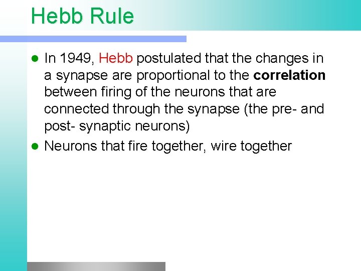
Hebb Rule In 1949, Hebb postulated that the changes in a synapse are proportional to the correlation between firing of the neurons that are connected through the synapse (the pre- and post- synaptic neurons) l Neurons that fire together, wire together l

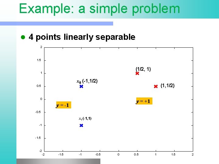
Example: a simple problem l 4 points linearly separable 2 1. 5 (1/2, 1) 1 x 0 (-1, 1/2) 0. 5 (1, 1/2) 0 y = +1 y = -1 -0. 5 x 1 (-1, 1) -1 -1. 5 -2 -2 -1. 5 -1 -0. 5 0 0. 5 1 1. 5 2

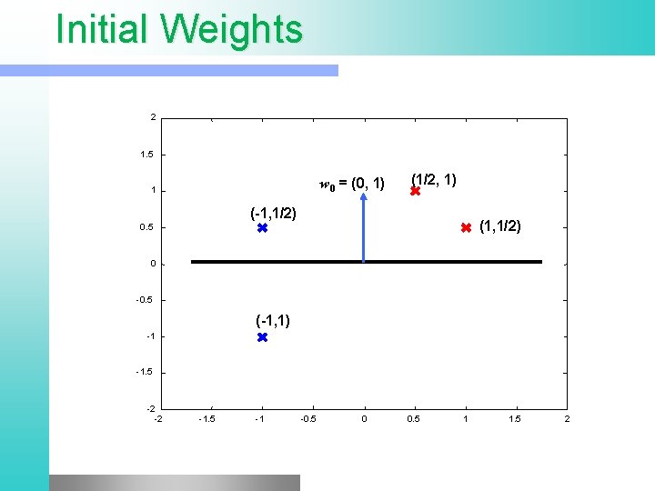
Initial Weights 2 1. 5 w 0 = (0, 1) 1 (1/2, 1) (-1, 1/2) (1, 1/2) 0. 5 0 -0. 5 (-1, 1) -1 -1. 5 -2 -2 -1. 5 -1 -0. 5 0 0. 5 1 1. 5 2

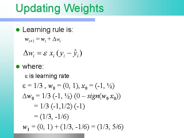
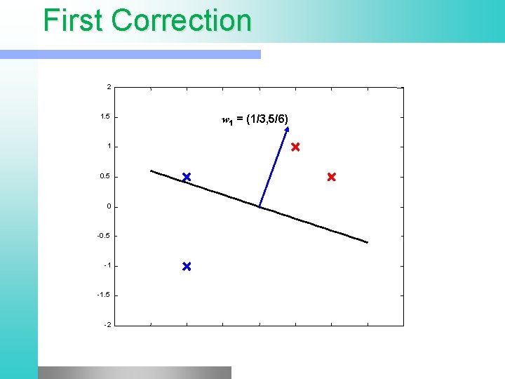
Updating Weights l Learning rule is: wi+1 = wi + Dwi l where: e is learning rate e = 1/3 , w 0 = (0, 1), x 0 = (-1, ½) Dw 0 = 1/3 (-1, ½) (0 – sign(w 0 x 0)) = 1/3 (-1, 1/2) (-1) = (1/3, -1/6) w 1 = (0, 1) + (1/3, -1/6) = (1/3, 5/6)

First Correction 2 1. 5 1 0. 5 0 -0. 5 -1 -1. 5 -2 w 1 = (1/3, 5/6)

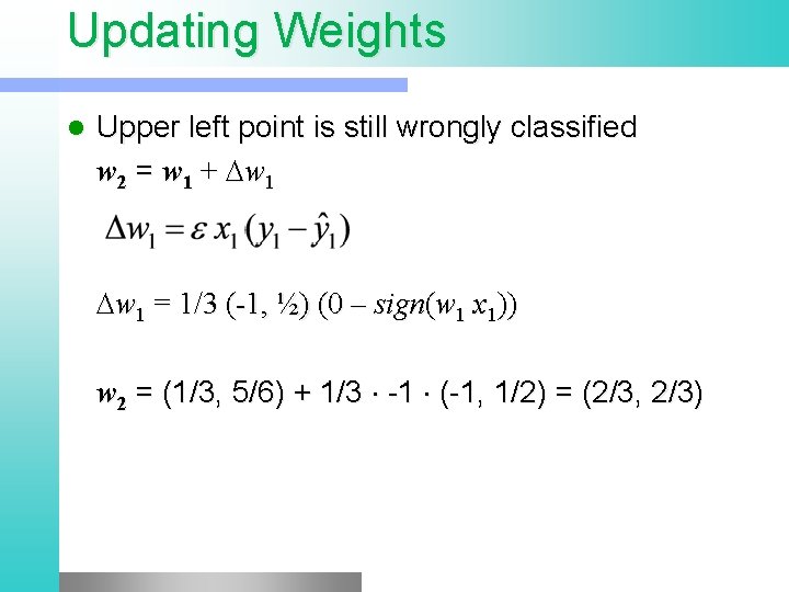
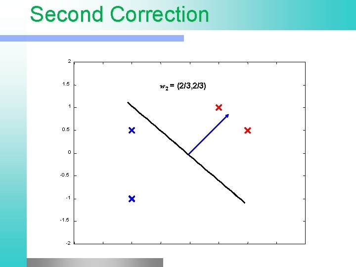
Updating Weights l Upper left point is still wrongly classified w 2 = w 1 + Dw 1 = 1/3 (-1, ½) (0 – sign(w 1 x 1)) w 2 = (1/3, 5/6) + 1/3 -1 (-1, 1/2) = (2/3, 2/3)

Second Correction 2 1. 5 1 0. 5 0 -0. 5 -1 -1. 5 -2 w 2 = (2/3, 2/3)

Example All 4 points are classified correctly l Toy problem – only 2 updates required l Correction of weights was simply a rotation of the separating hyper plane l Rotation can be applied to the right direction, but may require many updates l

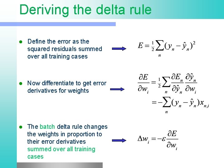
Deriving the delta rule l Define the error as the squared residuals summed over all training cases l Now differentiate to get error derivatives for weights l The batch delta rule changes the weights in proportion to their error derivatives summed over all training cases

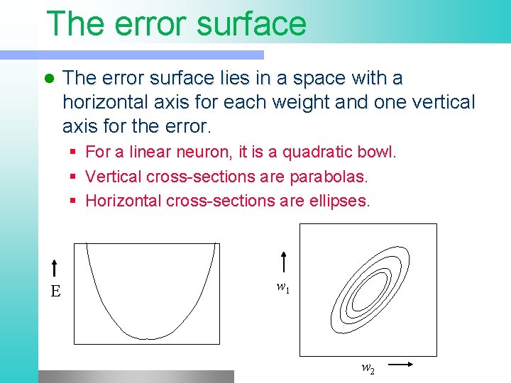
The error surface lies in a space with a horizontal axis for each weight and one vertical axis for the error. § For a linear neuron, it is a quadratic bowl. § Vertical cross-sections are parabolas. § Horizontal cross-sections are ellipses. E w 1 w 2

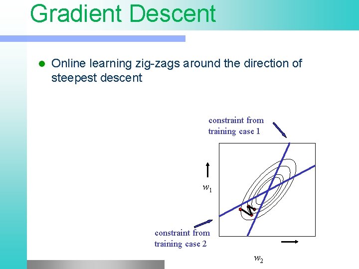
Gradient Descent l Online learning zig-zags around the direction of steepest descent constraint from training case 1 w 1 constraint from training case 2 w 2

Support Vector Machines

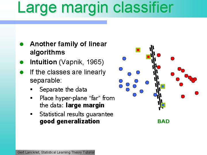
Large margin classifier Another family of linear algorithms l Intuition (Vapnik, 1965) l If the classes are linearly separable: l § § § Separate the data Place hyper-plane “far” from the data: large margin Statistical results guarantee good generalization Gert Lanckriet, Statistical Learning Theory Tutorial BAD

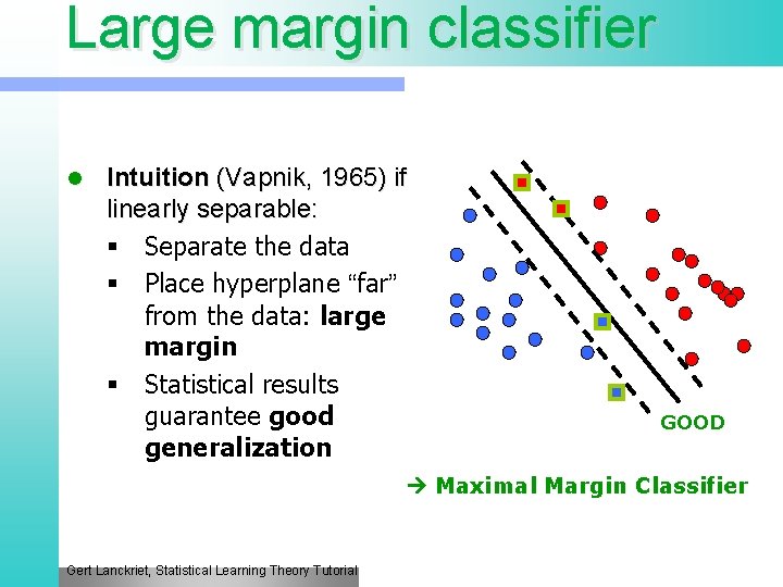
Large margin classifier l Intuition (Vapnik, 1965) if linearly separable: § Separate the data § Place hyperplane “far” from the data: large margin § Statistical results guarantee good generalization GOOD Maximal Margin Classifier Gert Lanckriet, Statistical Learning Theory Tutorial

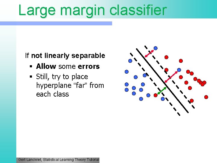
Large margin classifier If not linearly separable § Allow some errors § Still, try to place hyperplane “far” from each class Gert Lanckriet, Statistical Learning Theory Tutorial

Large Margin Classifiers l Advantages § Theoretically better (better error bounds) l Limitations § Computationally more expensive, large quadratic programming

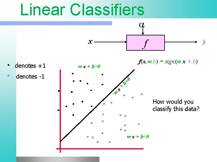
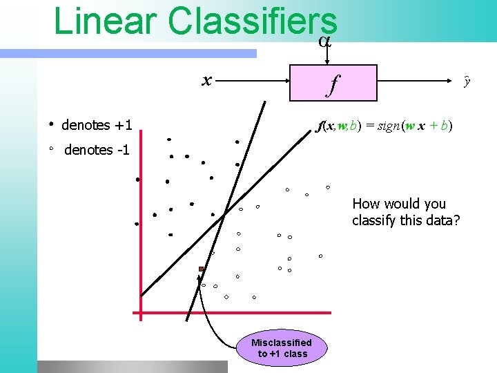
Linear Classifiers x denotes +1 f y f(x, w, b) = sign(w x + b) w x + b>0 w x + b= 0 denotes -1 How would you classify this data? w x + b<0

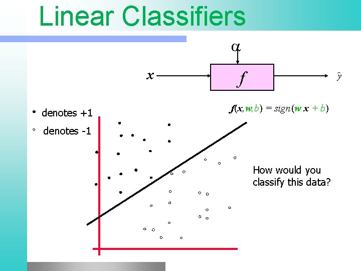
Linear Classifiers x denotes +1 f y f(x, w, b) = sign(w x + b) denotes -1 How would you classify this data?

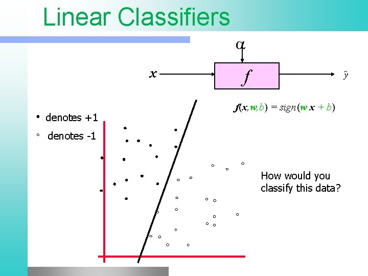
Linear Classifiers x denotes +1 f y f(x, w, b) = sign(w x + b) denotes -1 How would you classify this data?

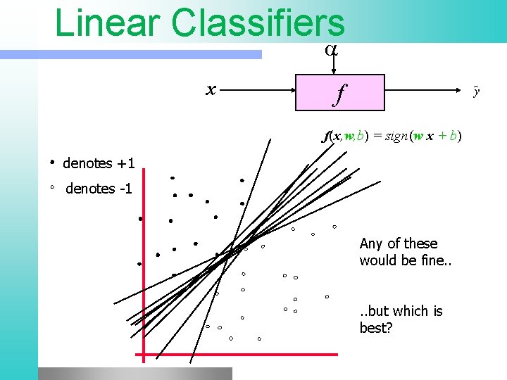
Linear Classifiers x f y f(x, w, b) = sign(w x + b) denotes +1 denotes -1 Any of these would be fine. . but which is best?

Linear Classifiers x f denotes +1 y f(x, w, b) = sign(w x + b) denotes -1 How would you classify this data? Misclassified to +1 class

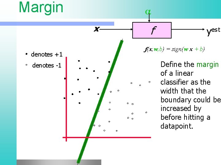
Margin x denotes +1 denotes -1 f yest f(x, w, b) = sign(w x + b) Define the margin of a linear classifier as the width that the boundary could be increased by before hitting a datapoint.

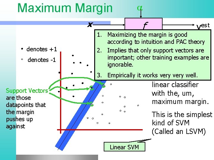
Maximum Margin x denotes +1 denotes -1 Support Vectors are those datapoints that the margin pushes up against f yest 1. Maximizing the margin is good accordingf(x, w, b) to intuition and PAC theory = sign(w x+ b) 2. Implies that only support vectors are important; other The training examples are maximum ignorable. margin linear 3. Empirically it works veryiswell. classifier the linear classifier with the, um, maximum margin. This is the simplest kind of SVM (Called an LSVM) Linear SVM

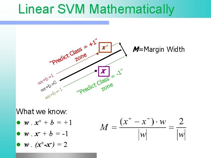
Linear SVM Mathematically 1” + + x = s s la e C t ic zon d e “Pr X- =1 +b x w =0 b + -1 wx = +b x w What we know: l w. x+ + b = +1 l w. x- + b = -1 l w. (x+-x-) = 2 M=Margin Width 1” = “P ss a l t C one c i z red

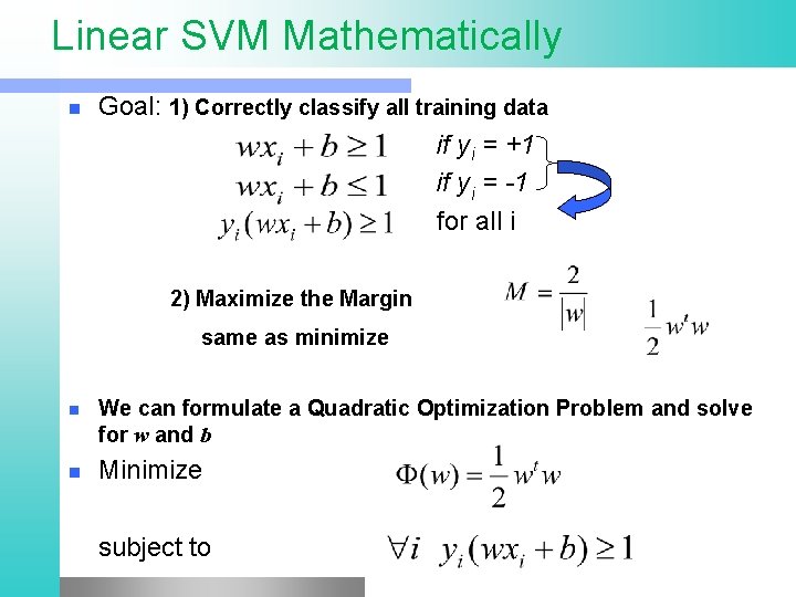
Linear SVM Mathematically Goal: 1) Correctly classify all training data if y i = +1 if y i = -1 for all i 2) Maximize the Margin same as minimize n n n We can formulate a Quadratic Optimization Problem and solve for w and b Minimize subject to

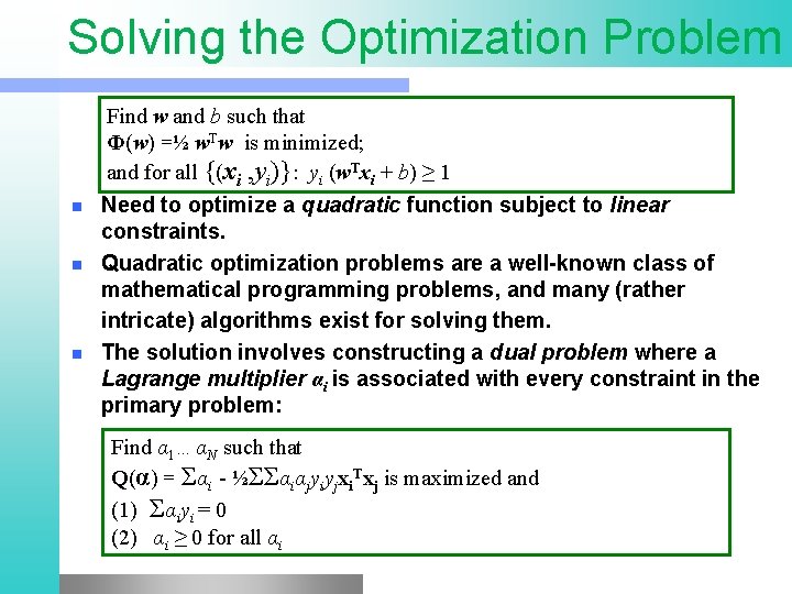
Solving the Optimization Problem n n n Find w and b such that Φ(w) =½ w. Tw is minimized; and for all {(xi , yi)}: yi (w. Txi + b) ≥ 1 Need to optimize a quadratic function subject to linear constraints. Quadratic optimization problems are a well-known class of mathematical programming problems, and many (rather intricate) algorithms exist for solving them. The solution involves constructing a dual problem where a Lagrange multiplier αi is associated with every constraint in the primary problem: Find α 1…αN such that Q(α) = Σαi - ½ΣΣαiαjyiyjxi. Txj is maximized and (1) Σαiyi = 0 (2) αi ≥ 0 for all αi

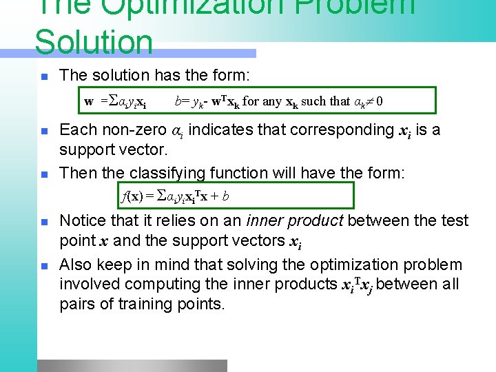
The Optimization Problem Solution n The solution has the form: w =Σαiyixi n n b= yk- w. Txk for any xk such that αk 0 Each non-zero αi indicates that corresponding xi is a support vector. Then the classifying function will have the form: f(x) = Σαiyixi. Tx + b Notice that it relies on an inner product between the test point x and the support vectors xi Also keep in mind that solving the optimization problem involved computing the inner products xi. Txj between all pairs of training points.

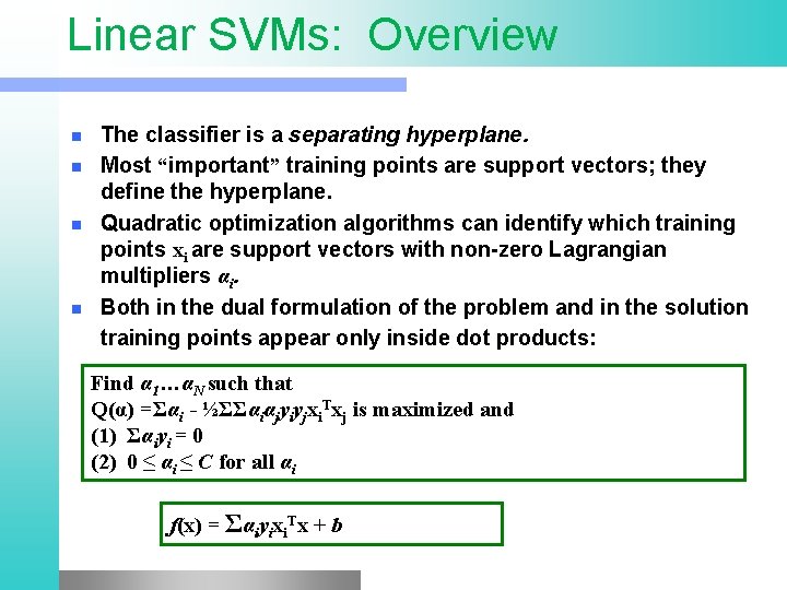
Linear SVMs: Overview n n The classifier is a separating hyperplane. Most “important” training points are support vectors; they define the hyperplane. Quadratic optimization algorithms can identify which training points xi are support vectors with non-zero Lagrangian multipliers αi. Both in the dual formulation of the problem and in the solution training points appear only inside dot products: Find α 1…αN such that Q(α) =Σαi - ½ΣΣαiαjyiyjxi. Txj is maximized and (1) Σαiyi = 0 (2) 0 ≤ αi ≤ C for all αi f(x) = Σαiyixi. Tx + b

Non Linear problem

Non Linear problem

Non Linear problem l l Kernel methods A family of non-linear algorithms Transform the non linear problem in a linear one (in a different feature space) Use linear algorithms to solve the linear problem in the new space Gert Lanckriet, Statistical Learning Theory Tutorial

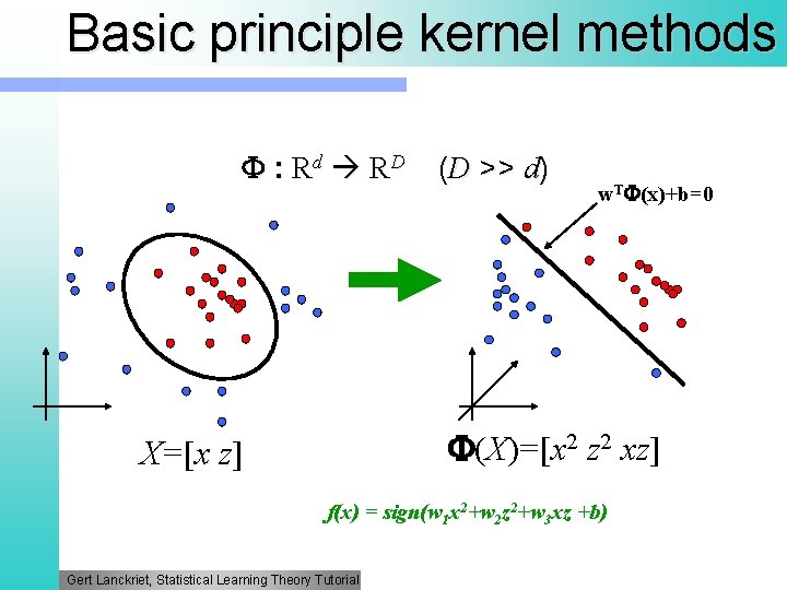
Basic principle kernel methods : Rd RD (D >> d) w. T (x)+b=0 (X)=[x 2 z 2 xz] X=[x z] f(x) = sign(w 1 x 2+w 2 z 2+w 3 xz +b) Gert Lanckriet, Statistical Learning Theory Tutorial

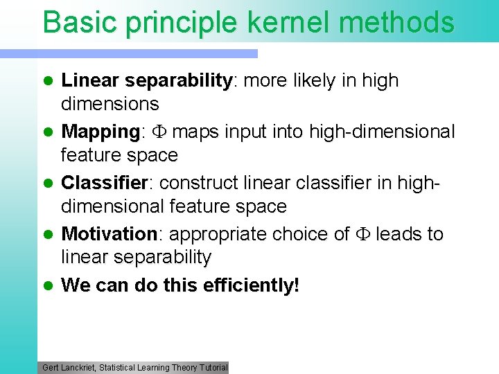
Basic principle kernel methods l l l Linear separability: more likely in high dimensions Mapping: maps input into high-dimensional feature space Classifier: construct linear classifier in highdimensional feature space Motivation: appropriate choice of leads to linear separability We can do this efficiently! Gert Lanckriet, Statistical Learning Theory Tutorial

Basic principle kernel methods l We can use the linear algorithms seen before (for example, perceptron) for classification in the higher dimensional space

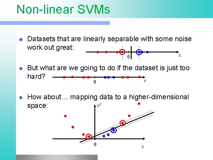
Non-linear SVMs n Datasets that are linearly separable with some noise work out great: x 0 n But what are we going to do if the dataset is just too hard? x 0 n How about… mapping data to a higher-dimensional x 2 space: 0 x

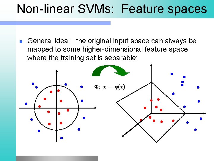
Non-linear SVMs: Feature spaces n General idea: the original input space can always be mapped to some higher-dimensional feature space where the training set is separable: Φ: x → φ(x)

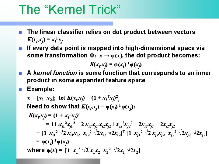
The “Kernel Trick” n n The linear classifier relies on dot product between vectors K(xi, xj) = xi. Txj If every data point is mapped into high-dimensional space via some transformation Φ: x → φ(x), the dot product becomes: K(xi, xj) = φ(xi) Tφ(xj) A kernel function is some function that corresponds to an inner product in some expanded feature space Example: x = [x 1 x 2]; let K(xi, xj) = (1 + xi. Txj)2, Need to show that K(xi, xj) = φ(xi) Tφ(xj): K(xi, xj) = (1 + xi. Txj)2 = 1+ xi 12 xj 12 + 2 xi 1 xj 1 xi 2 xj 2+ xi 22 xj 22 + 2 xi 1 xj 1 + 2 xi 2 xj 2 = [1 xi 12 √ 2 xi 1 xi 22 √ 2 xi 1 √ 2 xi 2]T [1 xj 12 √ 2 xj 1 xj 22 √ 2 xj 1 √ 2 xj 2] = φ(xi) Tφ(xj) where φ(x) = [1 x 12 √ 2 x 1 x 2 x 22 √ 2 x 1 √ 2 x 2]

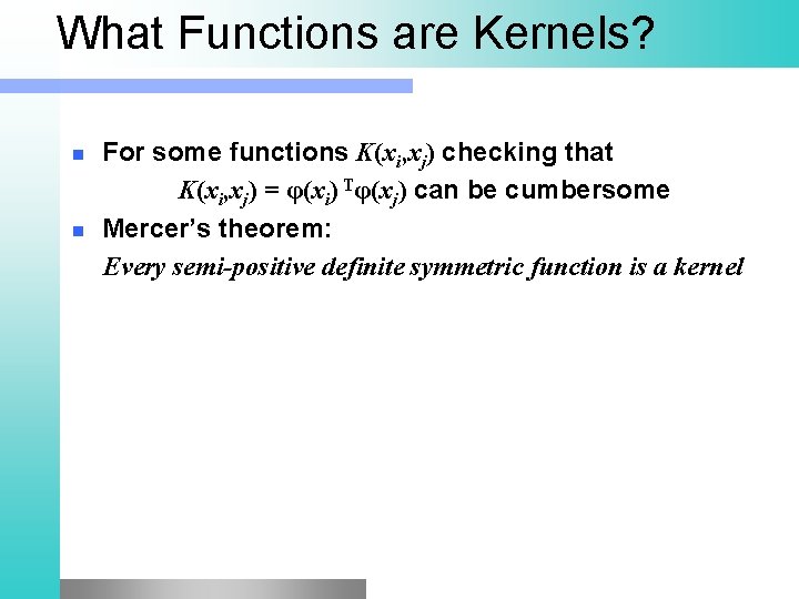
What Functions are Kernels? n n For some functions K(xi, xj) checking that K(xi, xj) = φ(xi) Tφ(xj) can be cumbersome Mercer’s theorem: Every semi-positive definite symmetric function is a kernel

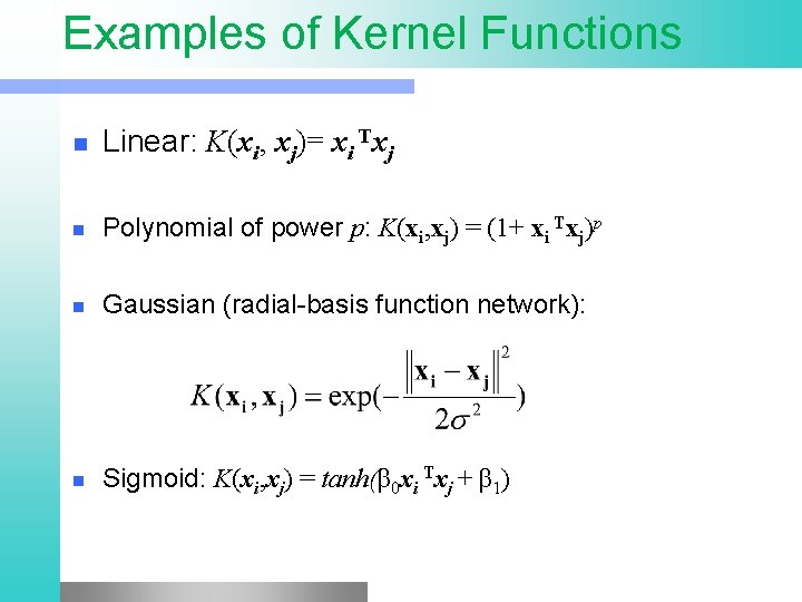
Examples of Kernel Functions n Linear: K(xi, xj)= xi Txj n Polynomial of power p: K(xi, xj) = (1+ xi Txj)p n Gaussian (radial-basis function network): n Sigmoid: K(xi, xj) = tanh(β 0 xi Txj + β 1)

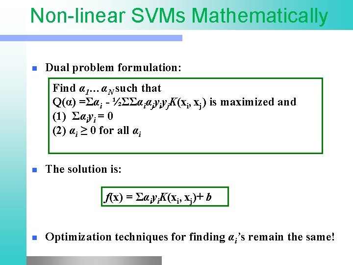
Non-linear SVMs Mathematically n Dual problem formulation: Find α 1…αN such that Q(α) =Σαi - ½ΣΣαiαjyiyj. K(xi, xj) is maximized and (1) Σαiyi = 0 (2) αi ≥ 0 for all αi n The solution is: f(x) = Σαiyi. K(xi, xj)+ b n Optimization techniques for finding αi’s remain the same!

Nonlinear SVM - Overview n n n SVM locates a separating hyperplane in the feature space and classify points in that space It does not need to represent the space explicitly, simply by defining a kernel function The kernel function plays the role of the dot product in the feature space.

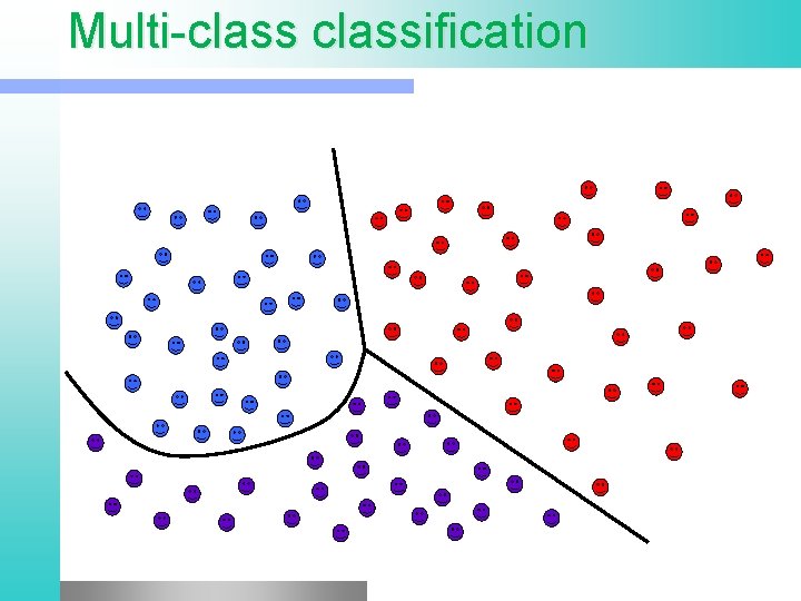
Multi-classification Given: some data items that belong to one of M possible classes l Task: Train the classifier and predict the class for a new data item l Geometrically: harder problem, no more simple geometry l

Multi-classification

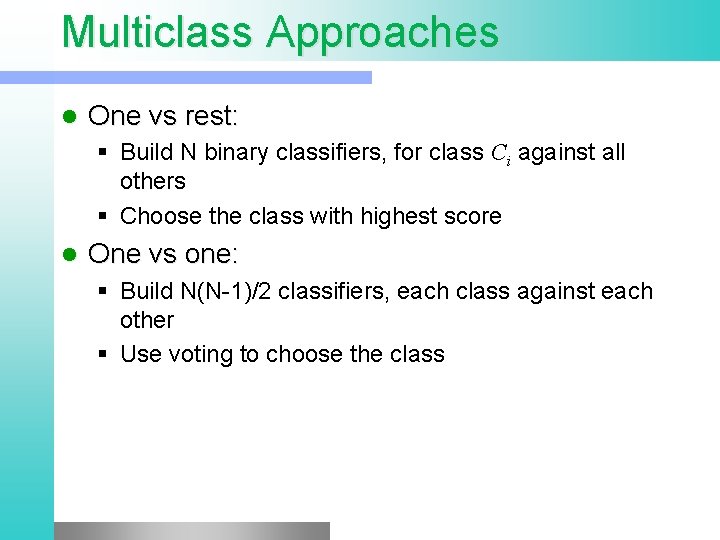
Multiclass Approaches l One vs rest: § Build N binary classifiers, for class Ci against all others § Choose the class with highest score l One vs one: § Build N(N-1)/2 classifiers, each class against each other § Use voting to choose the class

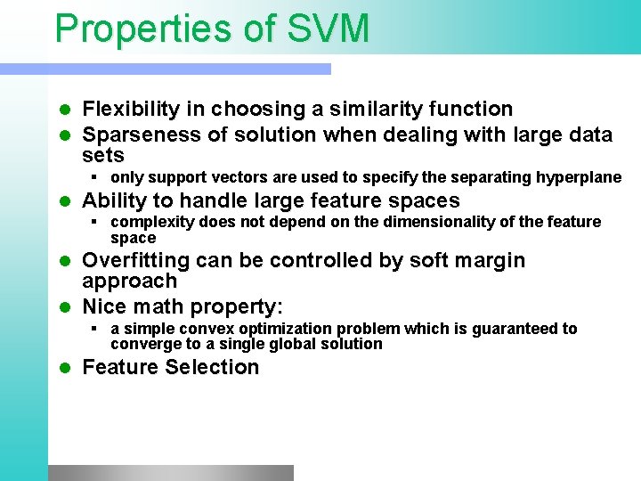
Properties of SVM l l Flexibility in choosing a similarity function Sparseness of solution when dealing with large data sets § only support vectors are used to specify the separating hyperplane l Ability to handle large feature spaces § complexity does not depend on the dimensionality of the feature space Overfitting can be controlled by soft margin approach l Nice math property: l § a simple convex optimization problem which is guaranteed to converge to a single global solution l Feature Selection

SVM Applications l SVM has been used successfully in many real-world problems § text (and hypertext) categorization § image classification – different types of subproblems § bioinformatics (protein classification, cancer classification) § hand-written character recognition

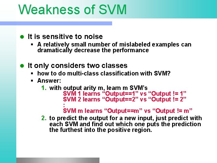
Weakness of SVM l It is sensitive to noise § A relatively small number of mislabeled examples can dramatically decrease the performance l It only considers two classes § how to do multi-classification with SVM? § Answer: 1. with output arity m, learn m SVM’s SVM 1 learns “Output==1” vs “Output != 1” SVM 2 learns “Output==2” vs “Output != 2” : SVM m learns “Output==m” vs “Output != m” 2. to predict the output for a new input, just predict with each SVM and find out which one puts the prediction the furthest into the positive region.

Application: Text Categorization l Task: The classification of natural text (or hypertext) documents into a fixed number of predefined categories based on their content. - email filtering, web searching, sorting documents by topic, etc. . l A document can be assigned to more than one category, so this can be viewed as a series of binary classification problems, one for each category

Application : Face Expression Recognition Construct feature space, by use of eigenvectors or other means l Multiple class problem, several expressions l Use multi-class SVM l

Some Issues l Choice of kernel - Gaussian or polynomial kernel is default - if ineffective, more elaborate kernels are needed l Choice of kernel parameters - e. g. σ in Gaussian kernel - σ is the distance between closest points with different classifications - In the absence of reliable criteria, applications rely on the use of a validation set or cross-validation to set such parameters. l Optimization criterion – Hard margin v. s. Soft margin - a lengthy series of experiments in which various parameters are tested

Additional Resources lib. SVM l An excellent tutorial on VC-dimension and Support Vector Machines: l C. J. C. Burges. A tutorial on support vector machines for pattern recognition. Data Mining and Knowledge Discovery, 2(2): 955 -974, 1998. The VC/SRM/SVM Bible: Statistical Learning Theory by Vladimir Vapnik, Wileyl Interscience; 1998 http: //www. kernel-machines. org/

Reference Support Vector Machine Classification of Microarray Gene Expression Data, Michael P. S. Brown William Noble Grundy, David Lin, Nello Cristianini, Charles Sugnet, Manuel Ares, Jr. , David Haussler l www. cs. utexas. edu/users/mooney/cs 391 L/svm. p pt l Text categorization with Support Vector Machines: learning with many relevant features T. Joachims, ECML - 98 l