Classification Dissimilarity measures Resemblance functions Cluster analysis TWINSPAN

Classification (Dis)similarity measures, Resemblance functions Cluster analysis TWINSPAN

Similarity measures Each ordination or classification method is based (explicitly or implicitly) on some similarity measure (Two possible formulations of ordination problem)

Similarities (dissimilarities, distances) Resemblance functions (the term includes both similarities and dissimilarities) If 0 ≤ S ≤ 1, then often D = 1 – S nebo D = √(1 – S) nebo D = √(1 – S 2) Different indices are usually used for sample similarity than for species similarity Similarity of two cases (samples) has a meaning by itself: similarity of two species has meaning only in relation to the data set. Species set is „fixed“ (e. g. all vascular plant species), cases are usually some selection from a “population of sites” (and the population of sites means geographic, environmental etc. definition of the set we are interested in).

Distance – should fulfill the triangular inequality C B A AB < AC + BC

Resemblance functions • Probably hundreds were proposed and tens are used We compare: Presence/absence Data type (0 / 1) Quantitative cases - Q species – R Sørensen coefficient Jaccard coefficient Pearson f (V) coeff. Yule (Q) coefficient Euclidean distance c 2 distance Percentage similarity correlation coefficients c 2 distance

Case similarity based on qualitative data Sörensen Jacquard d - number of species absent in both cases (usually not used) consequently, the value is independent of other cases in a table

Species similarity based on presence absence d - number of cases without both species - absolutely necessary

Species vs. case similarity • Species similarity (i. e. similarity of species ecological behavior, e. g. V, Q) – often scaled from -1 to 1. “Null model” means independence of the species, and in this case V=Q=0. • Case similarity (S, J), usually scaled from 0 (no common species) to 1 (identical species composition). No “null model” available. (or better, no meaningfull null model available; compare – random selection of two sets of species from species pool? )

Quantitative data Transformation is an algebraic function Xij’=f(Xij) which is applied independently of the other values. Standardization is done either with respect to the values of other species in the case (standardization by cases) or with respect to the values of the species in other cases (standardization by species). Centering means the subtraction of a mean so that the resulting variable (species) or case has a mean of zero. Standardization usually means division of each value by the case (species) norm or by the total of all the values in a case (species).

„Ordinal transformation“ of Br. -Bl. scale is roughly equivalent to log transformation of the cover values

Why to use the log(x) transformation • Changes the positively skewed distrnibution to (something closer to) symmetric – (in ordinations, not very relevant) • Changes multiplicativity to additivity • In effect, increases the effect of low abundant species, decreases the effect of dominants

x differ x log(x) 1 0 10 9 1 1 100 90 2 1

Why to use the log(ax+b) transformation • If x=0, log(x) is not defined • Log(ax+b) – if b=1, then the function is 0 for x=0 - reasonable option • Thus, why not simply log(x+1)? • If the X values are small, then:

log(x+1) 0. 35 0. 3 log(X+1) 0. 25 0. 2 0. 15 0. 1 0. 05 0 0. 00 0. 20 0. 40 0. 60 X 0. 80 1. 00 1. 20

log(10 x+1) 1. 2 log(10 X+1) 1 0. 8 0. 6 0. 4 0. 2 0 0. 00 0. 20 0. 40 0. 60 X 0. 80 1. 00 1. 20

log(100 x+1) 2. 5 log(100 X+1) 2 1. 5 1 0. 5 0 0. 00 0. 20 0. 40 0. 60 X 0. 80 1. 00 1. 20

Euclidean distance For ED, standardize by case norm, not by total The cases with t contain values standardized by the total, those with n are standardized by case norm. For cases standardized by total, ED 12 = 1. 41 (√ 2), whereas ED 34=0. 82, whereas for cases standardized by case norm, ED 12=ED 34=1. 41

Euclidean distance after standardization by sample norm – ‚chord distance“ http: //www. umass. edu/landeco/teaching/multivariate/readings/Mc. Cune. and. Grace. 2002. chapter 6. pdf

Percentual similarity (quantitative Sörensen) Neither ED, nor PS take into consideration species which are absent in the two compared cases

PS – often multiplied by 100(%) Bray-Curtis distance = 1 – PS Often used with standardization by sample total

Similarity of species based on quantitative data Correlation coefficients (ordinary, rank) – i. e. again taking into account the cases where both species are missing Note the implicit double standardization (by both, case and species total) Consequently, the value is changing according to composition of other cases in the total table.

Similarity of samples vs. similarity of communities Inspired be seemingly high beta-diversity of insects in tropics

Normalized expected shared species = expected number of shared species in two subsamples taken randomly from the second sample. 2 2

Similarity of objects when variable are measured on various scales •

Gower distance •

Standardization of variables by the s. d. or range is sometimes problematic – possibility to standardize by variation – see Lepš et al. 2006

Similarity matrices - directly used in Multidimensional scaling (both metric and non-metric – see Šmilauer lecture) Mantel test

Mantel Test • Question – is there any dependence between two (dis)similarity matrices? • e. g. is the distance of individual plants in physical space correlated with their genetic dissimilarity?

Individuals in the plot Indiv. No. 5 And this individual is strange (just one of five)

Two dissimilarity matrices Distance in the plot plant 1 2 Genetic distance 3 4 1 5 plant 1 2 3 4 1 2 1. 41 3 1. 00 2. 24 4 1. 00 1. 41 5 12. 04 10. 63 12. 73 11. 31 2 0. 1 3 0. 2 4 0. 1 0. 3 0. 2 5 0. 9 0. 6 0. 7 0. 8 5

Regression is highly significant (but we have 10 “independent” observations out of five plants!) And four „independent“ observations out of ten are the largest

Solution • Permutation test • Not individual distances, but individuals are permuted

Classification Of historical significance only

Non-hierarchical classification • K-means clustering • In fact, „reverse“ ANOVA • ANOVA: F=Msgroup/MSresidual • The goal – divide the set into groups to maximize F (multivariate counterpart of F)

Hierarchical agglomerative (cluster analysis)

Subjective decisions in the objective procedure Nevertheless, the procedure is reproducible

Cluster analysis joining Distances among objects are in the (dis)similarity matrix. In the hierarchical classification, we need also the distances among clusters. .

Single linkage (nearest neighbour, representative of short hand) and complete linkage (furthest neighbour, representative of long hand methods) Several other methods, e. g. Ward (minimum dispersion), “average linkage” – most popular, but the term was used for several methods – preferred name UPGMA - Unweighted Pair Group Method with Arithmetic mean

Single linkage - > chaining

Order does not play a role

TWINSPAN – Two Way INdicator SPecies ANalysis • Invented (by Mark Hill) to search for a pattern in extensive vegetation tables • Inspired by classical phytosociology • Algorithm based on the presence/absence data • Quantitative data used for definition of “pseudospecies”

TWINSPAN 2 - pseudospecies Lower exclusive border • Definition of cut levels has similar effect as transformation (weighting dominance vs. presence/absence) • Compare 0, 1, 100 vs. 0, 10, 20, 30, 40

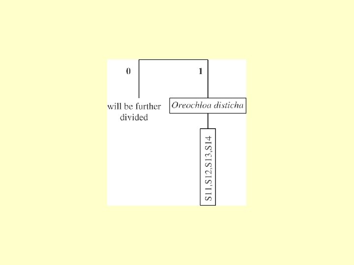
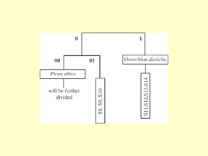
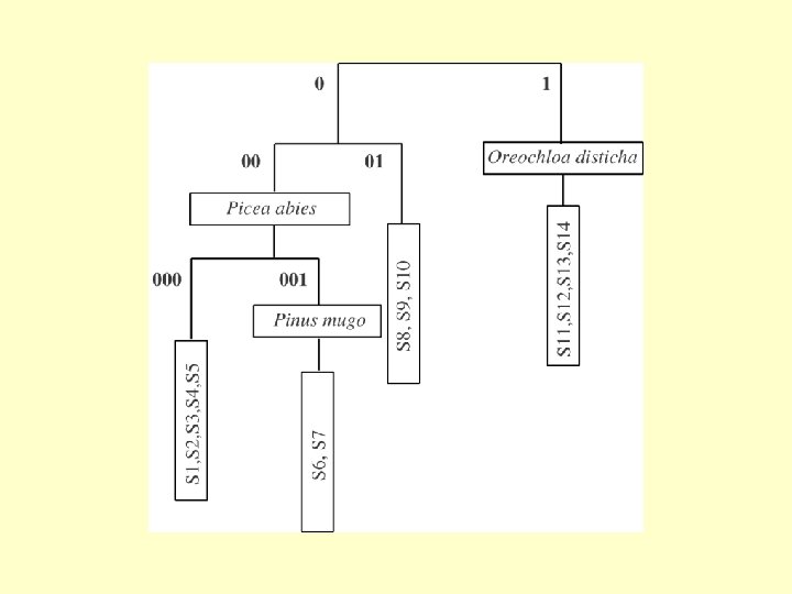
Divisive method – each group is divided on the basis of the first CA axis The first axis is based on CA ordination - it is then not surprising, that TWINSPAN results well correspond to, e. g. , DCA and individual groups are well clustered in ordination space.

Divisive method – each group is divided on the basis of the first CA axis Most of the cases are usually around the center -> we need some polarization

Polarized ordination (based on “indicator species”)

01 is more similar to 1 than 00 The order of groups reflects possible gradient in the table