Classification Definition n Given a collection of records

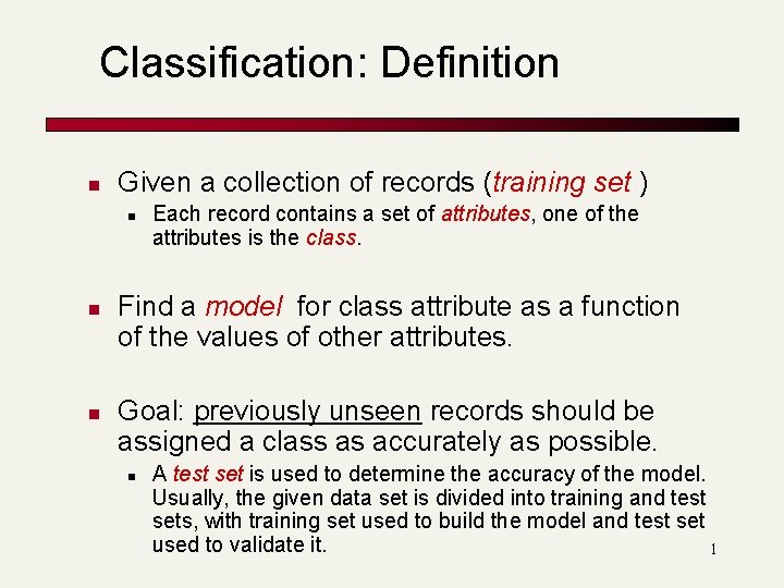
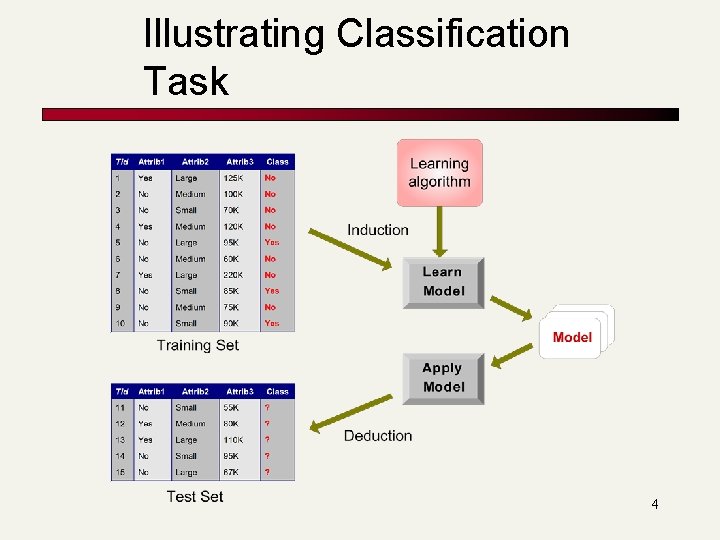
Classification: Definition n Given a collection of records (training set ) n n n Each record contains a set of attributes, one of the attributes is the class. Find a model for class attribute as a function of the values of other attributes. Goal: previously unseen records should be assigned a class as accurately as possible. n A test set is used to determine the accuracy of the model. Usually, the given data set is divided into training and test sets, with training set used to build the model and test set used to validate it. 1

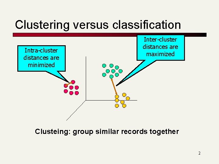
Clustering versus classification Intra-cluster distances are minimized Inter-cluster distances are maximized Clusteing: group similar records together 2

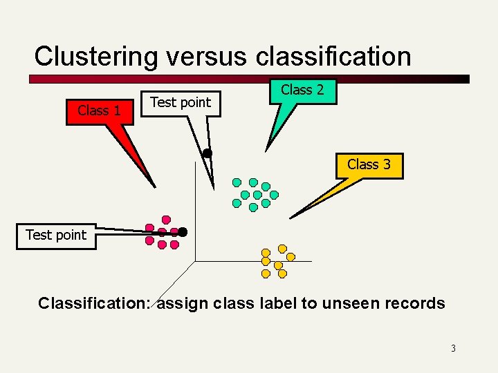
Clustering versus classification Class 1 Test point Class 2 Class 3 Test point Classification: assign class label to unseen records 3

Illustrating Classification Task 4

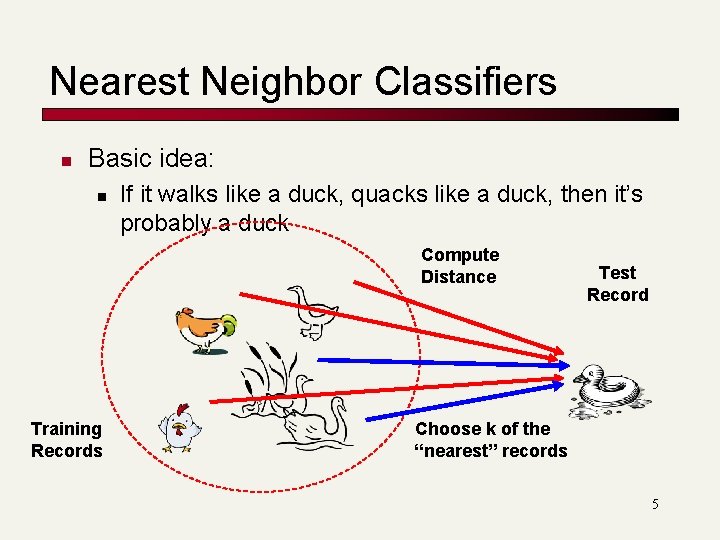
Nearest Neighbor Classifiers n Basic idea: n If it walks like a duck, quacks like a duck, then it’s probably a duck Compute Distance Training Records Test Record Choose k of the “nearest” records 5

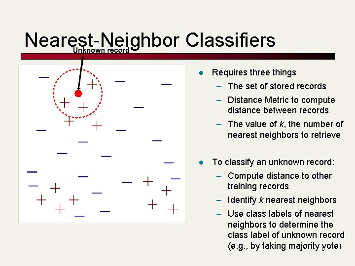
Nearest-Neighbor Classifiers l Requires three things – The set of stored records – Distance Metric to compute distance between records – The value of k, the number of nearest neighbors to retrieve l To classify an unknown record: – Compute distance to other training records – Identify k nearest neighbors – Use class labels of nearest neighbors to determine the class label of unknown record (e. g. , by taking majority 6 vote)

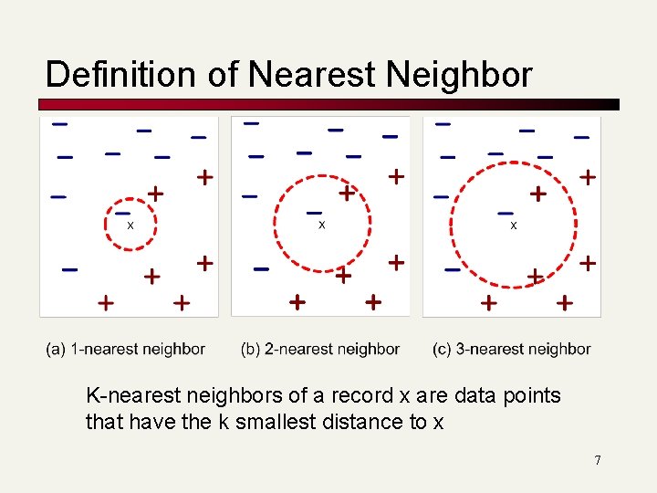
Definition of Nearest Neighbor K-nearest neighbors of a record x are data points that have the k smallest distance to x 7

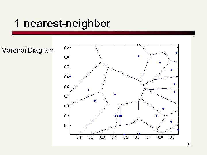
1 nearest-neighbor Voronoi Diagram 8

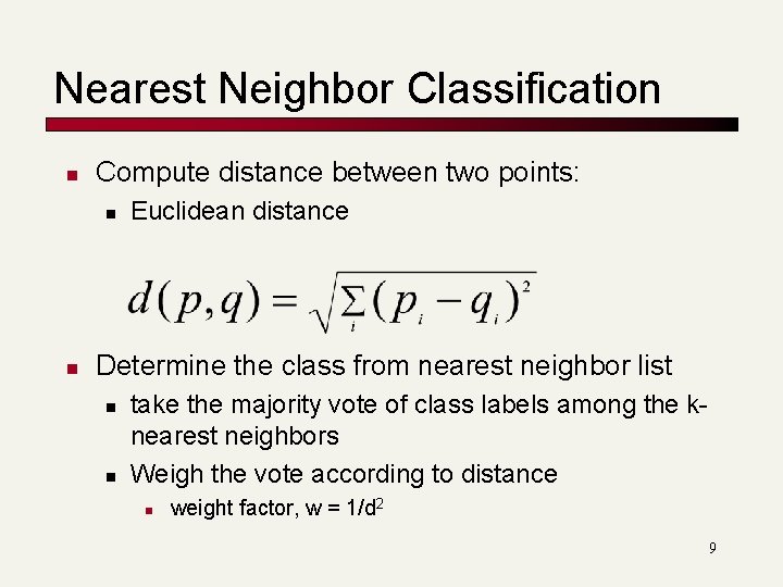
Nearest Neighbor Classification n Compute distance between two points: n n Euclidean distance Determine the class from nearest neighbor list n n take the majority vote of class labels among the knearest neighbors Weigh the vote according to distance n weight factor, w = 1/d 2 9

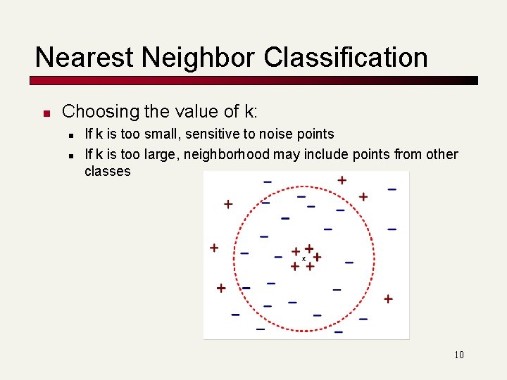
Nearest Neighbor Classification n Choosing the value of k: n n If k is too small, sensitive to noise points If k is too large, neighborhood may include points from other classes 10

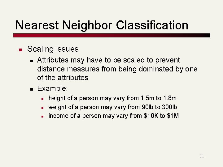
Nearest Neighbor Classification n Scaling issues n n Attributes may have to be scaled to prevent distance measures from being dominated by one of the attributes Example: n n n height of a person may vary from 1. 5 m to 1. 8 m weight of a person may vary from 90 lb to 300 lb income of a person may vary from $10 K to $1 M 11

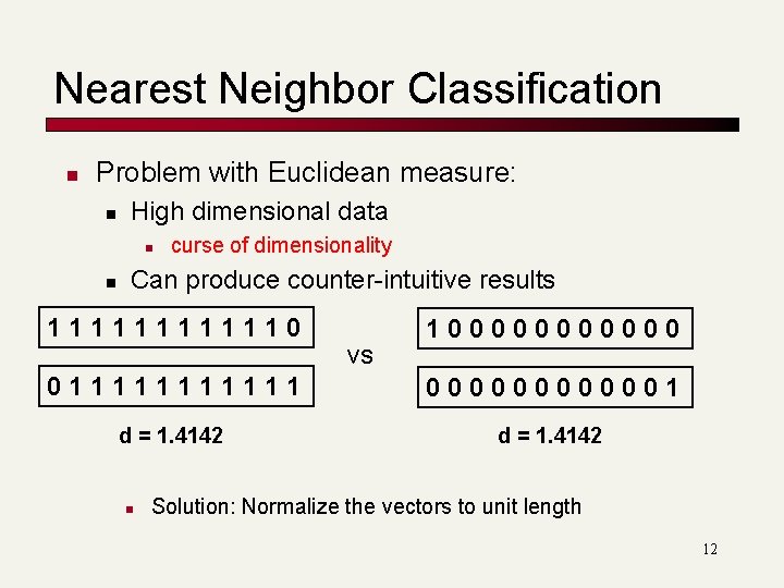
Nearest Neighbor Classification n Problem with Euclidean measure: n High dimensional data n n curse of dimensionality Can produce counter-intuitive results 1111110 vs 1000000 0111111 0000001 d = 1. 4142 n Solution: Normalize the vectors to unit length 12

Nearest neighbor Classification n k-NN classifiers are lazy learners n n It does not build models explicitly Classifying unknown records are relatively expensive 13

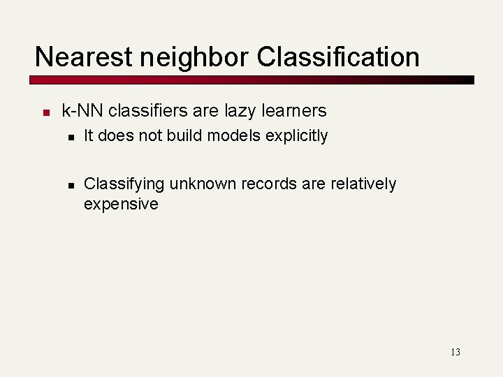
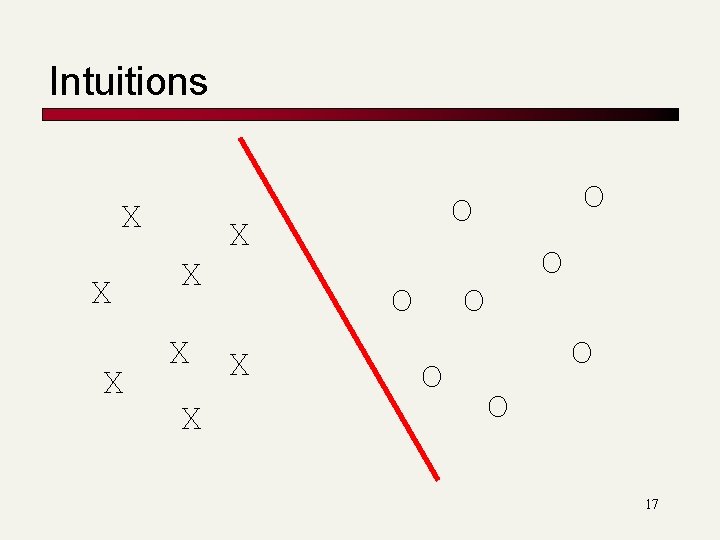
SVM-Intuitions X X X O X O O O 14

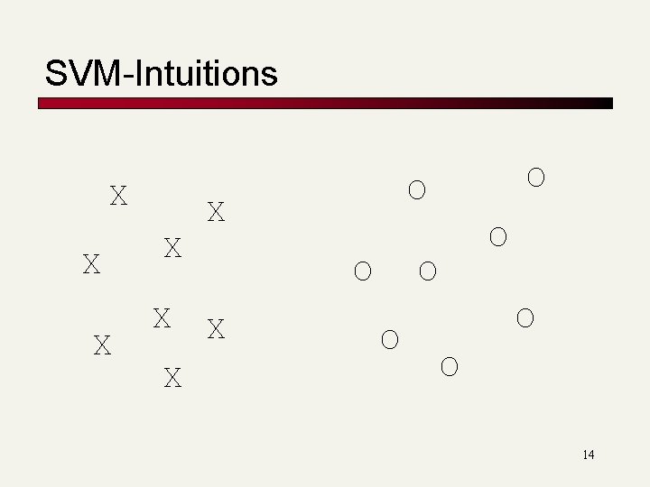
Intuitions X X X O X O O O 15

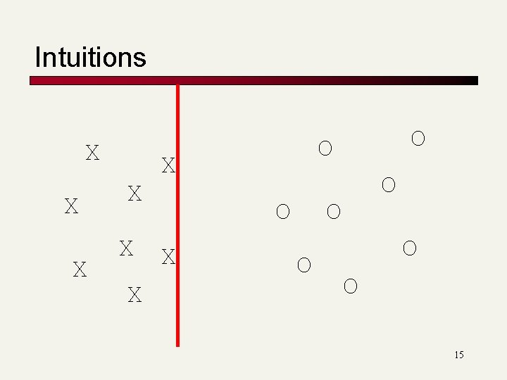
Intuitions X X X O X O O O 16

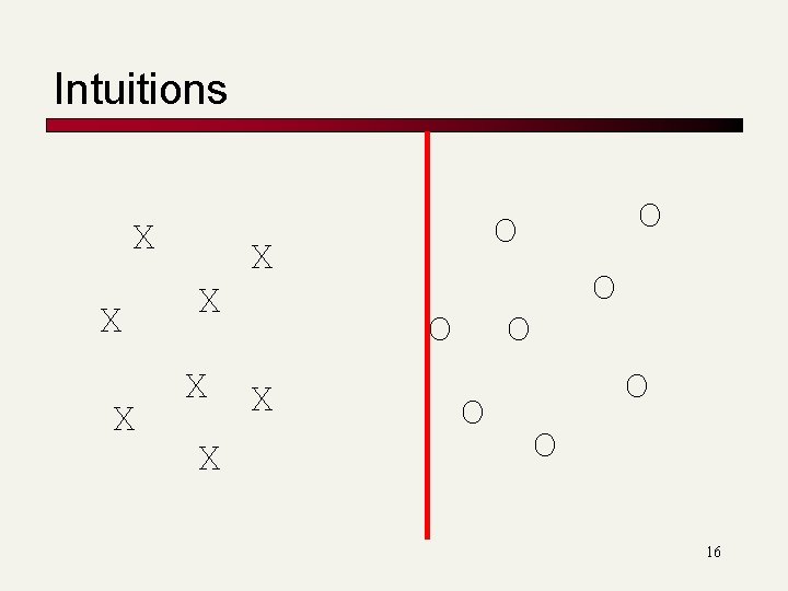
Intuitions X X X O X O O O 17

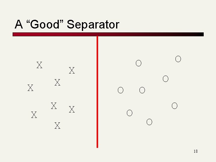
A “Good” Separator X X X O X O O O 18

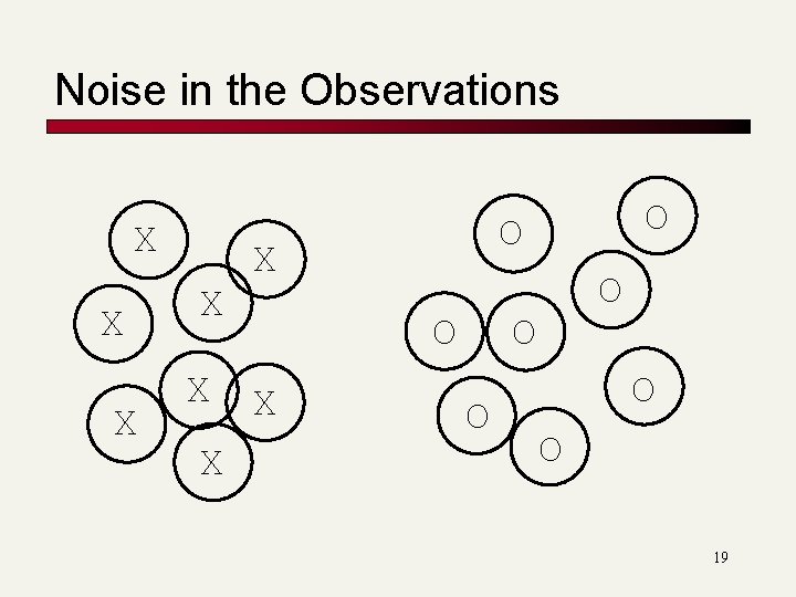
Noise in the Observations X X X O X O O O 19

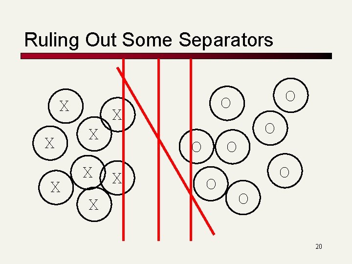
Ruling Out Some Separators X X X O X O O O 20

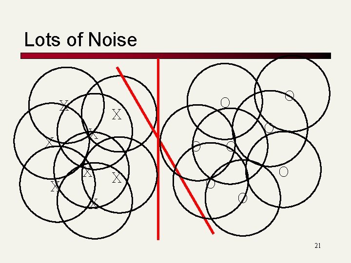
Lots of Noise X X X O X O O O 21

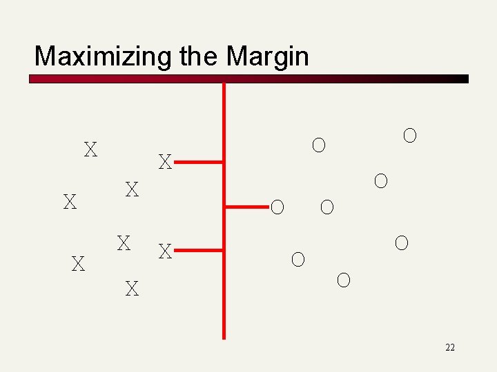
Maximizing the Margin X X X O X O O O 22

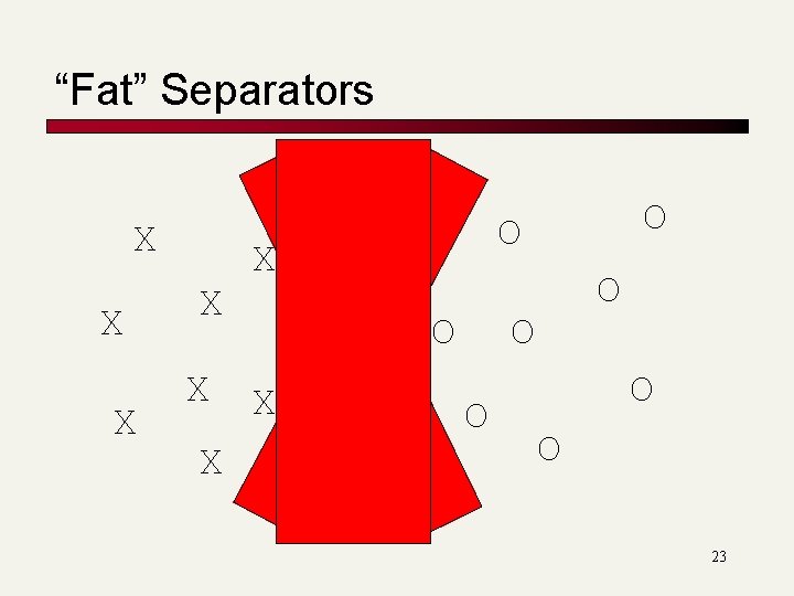
“Fat” Separators X X X O X O O O 23

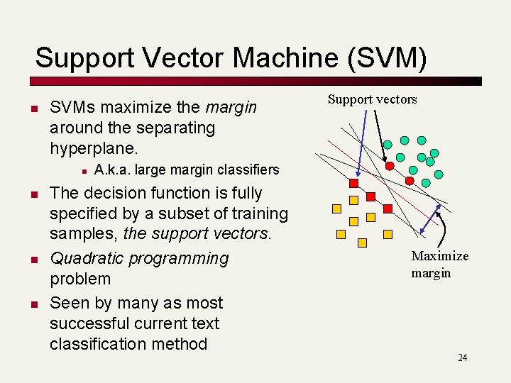
Support Vector Machine (SVM) n SVMs maximize the margin around the separating hyperplane. n n Support vectors A. k. a. large margin classifiers The decision function is fully specified by a subset of training samples, the support vectors. Quadratic programming problem Seen by many as most successful current text classification method Maximize margin 24

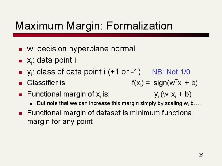
Maximum Margin: Formalization n w: decision hyperplane normal xi: data point i yi: class of data point i (+1 or -1) n Classifier is: n Functional margin of xi is: n n NB: Not 1/0 f(xi) = sign(w. Txi + b) yi (w. Txi + b) But note that we can increase this margin simply by scaling w, b…. Functional margin of dataset is minimum functional margin for any point 25

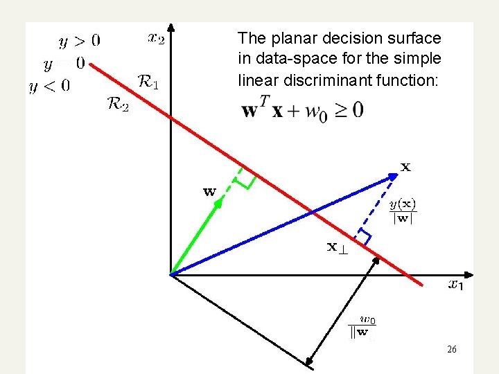
The planar decision surface in data-space for the simple linear discriminant function: 26

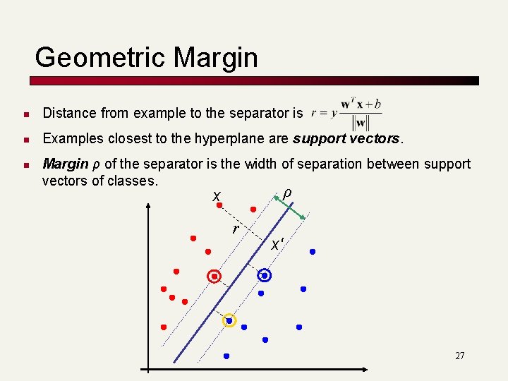
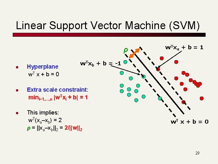
Geometric Margin n Distance from example to the separator is n Examples closest to the hyperplane are support vectors. n Margin ρ of the separator is the width of separation between support vectors of classes. ρ x r x′ 27

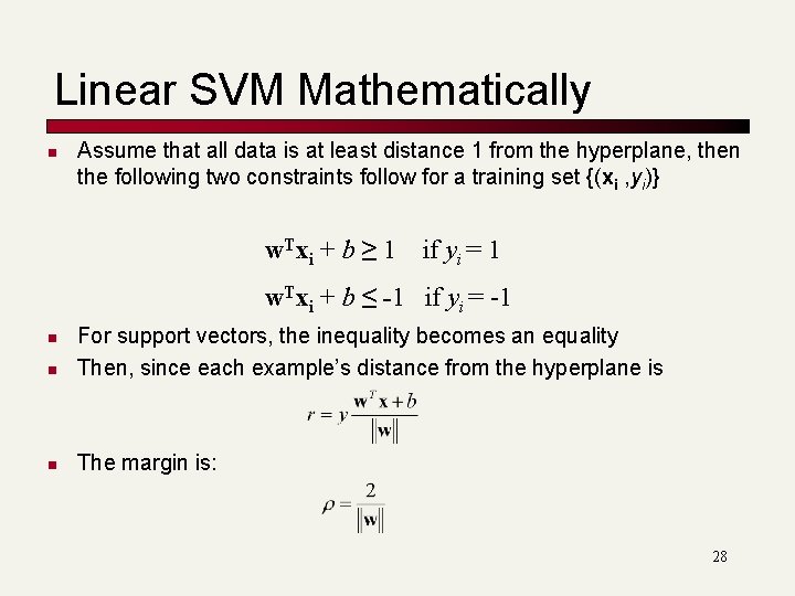
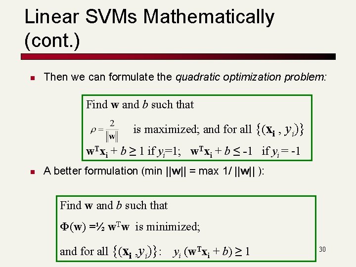
Linear SVM Mathematically n Assume that all data is at least distance 1 from the hyperplane, then the following two constraints follow for a training set {(xi , yi)} w. Txi + b ≥ 1 if yi = 1 w. Txi + b ≤ -1 if yi = -1 n For support vectors, the inequality becomes an equality Then, since each example’s distance from the hyperplane is n The margin is: n 28

Linear Support Vector Machine (SVM) ρ n n n Hyperplane w. T x + b = 0 w. T x a + b = 1 w. Txb + b = -1 Extra scale constraint: mini=1, …, n |w. Txi + b| = 1 This implies: w. T(xa–xb) = 2 ρ = ||xa–xb||2 = 2/||w||2 w. T x + b = 0 29

Linear SVMs Mathematically (cont. ) n Then we can formulate the quadratic optimization problem: Find w and b such that is maximized; and for all {(xi , yi)} w. Txi + b ≥ 1 if yi=1; w. Txi + b ≤ -1 if yi = -1 n A better formulation (min ||w|| = max 1/ ||w|| ): Find w and b such that Φ(w) =½ w. Tw is minimized; and for all {(xi , yi)}: yi (w. Txi + b) ≥ 1 30

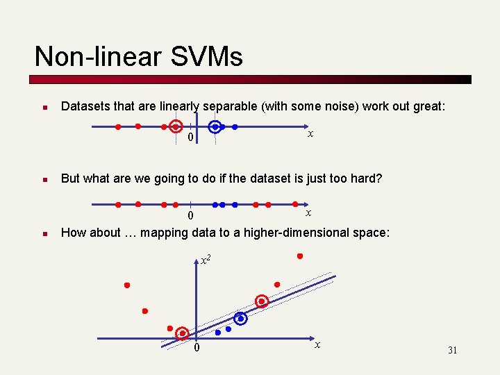
Non-linear SVMs n Datasets that are linearly separable (with some noise) work out great: x 0 n But what are we going to do if the dataset is just too hard? n x 0 How about … mapping data to a higher-dimensional space: x 2 0 x 31

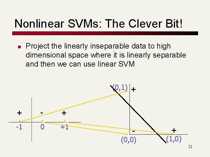
Nonlinear SVMs: The Clever Bit! n Project the linearly inseparable data to high dimensional space where it is linearly separable and then we can use linear SVM (0, 1) + + -1 0 +1 (0, 0) + (1, 0) 32

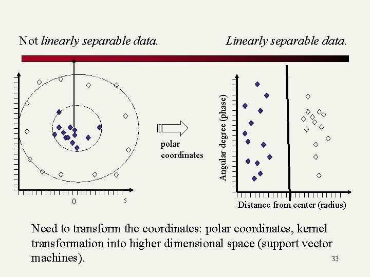
Linearly separable data. polar coordinates 0 5 Angular degree (phase) Not linearly separable data. Distance from center (radius) Need to transform the coordinates: polar coordinates, kernel transformation into higher dimensional space (support vector 33 machines).

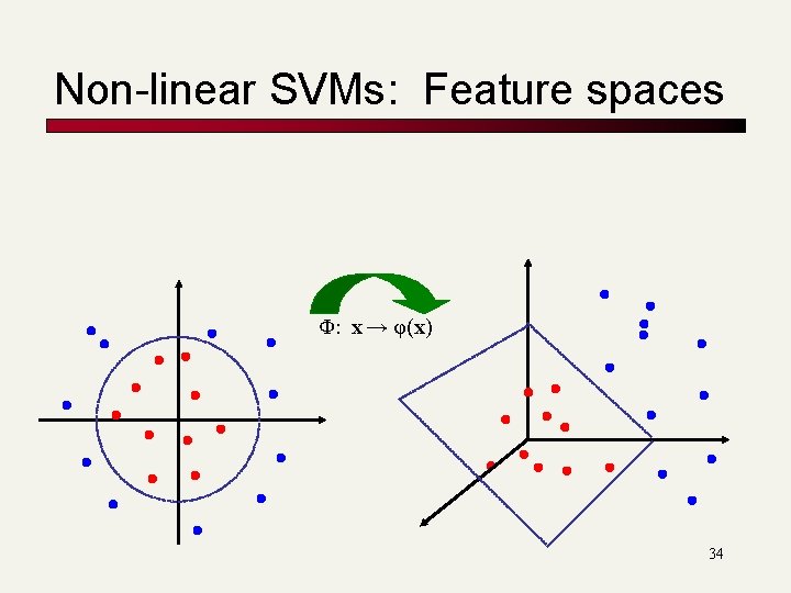
Non-linear SVMs: Feature spaces Φ: x → φ(x) 34

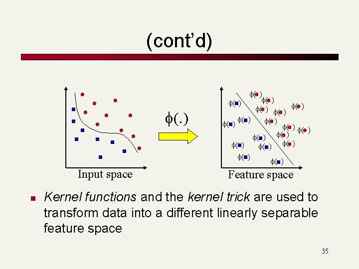
(cont’d) f(. ) Input space n f( ) f( ) f( ) f( ) f( ) Feature space Kernel functions and the kernel trick are used to transform data into a different linearly separable feature space 35

Mathematical Details : SKIP 36

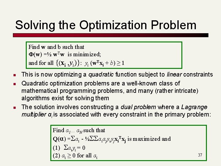
Solving the Optimization Problem Find w and b such that Φ(w) =½ w. Tw is minimized; and for all {(xi , yi)}: yi (w. Txi + b) ≥ 1 n n n This is now optimizing a quadratic function subject to linear constraints Quadratic optimization problems are a well-known class of mathematical programming problems, and many (rather intricate) algorithms exist for solving them The solution involves constructing a dual problem where a Lagrange multiplier αi is associated with every constraint in the primary problem: Find α 1…αN such that Q(α) =Σαi - ½ΣΣαiαjyiyjxi. Txj is maximized and (1) Σαiyi = 0 (2) αi ≥ 0 for all αi 37

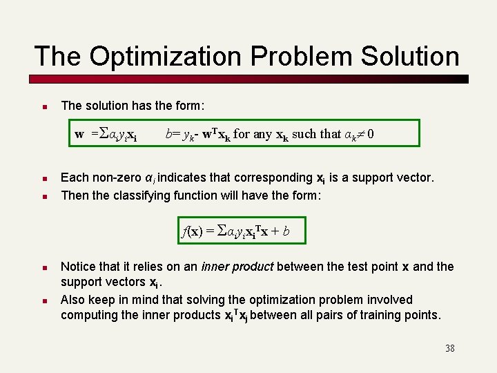
The Optimization Problem Solution n The solution has the form: w =Σαiyixi n n b= yk- w. Txk for any xk such that αk 0 Each non-zero αi indicates that corresponding xi is a support vector. Then the classifying function will have the form: f(x) = Σαiyixi. Tx + b n n Notice that it relies on an inner product between the test point x and the support vectors xi. Also keep in mind that solving the optimization problem involved computing the inner products xi. Txj between all pairs of training points. 38

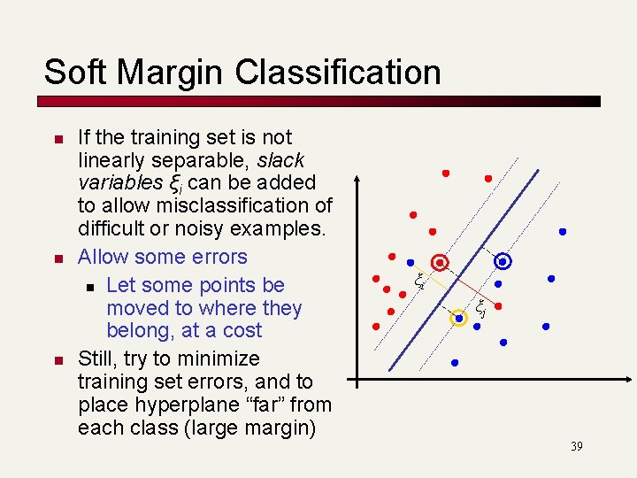
Soft Margin Classification n If the training set is not linearly separable, slack variables ξi can be added to allow misclassification of difficult or noisy examples. Allow some errors n Let some points be moved to where they belong, at a cost Still, try to minimize training set errors, and to place hyperplane “far” from each class (large margin) ξi ξj 39

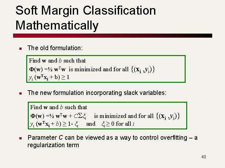
Soft Margin Classification Mathematically n The old formulation: Find w and b such that Φ(w) =½ w. Tw is minimized and for all {(xi yi (w. Txi + b) ≥ 1 n , yi)} The new formulation incorporating slack variables: Find w and b such that Φ(w) =½ w. Tw + CΣξi is minimized and for all {(xi yi (w. Txi + b) ≥ 1 - ξi and ξi ≥ 0 for all i n , yi)} Parameter C can be viewed as a way to control overfitting – a regularization term 40

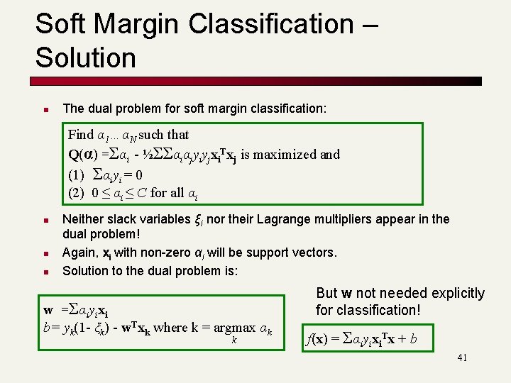
Soft Margin Classification – Solution n The dual problem for soft margin classification: Find α 1…αN such that Q(α) =Σαi - ½ΣΣαiαjyiyjxi. Txj is maximized and (1) Σαiyi = 0 (2) 0 ≤ αi ≤ C for all αi n n n Neither slack variables ξi nor their Lagrange multipliers appear in the dual problem! Again, xi with non-zero αi will be support vectors. Solution to the dual problem is: w =Σαiyixi b= yk(1 - ξk) - w. Txk where k = argmax αk k But w not needed explicitly for classification! f(x) = Σαiyixi. Tx + b 41

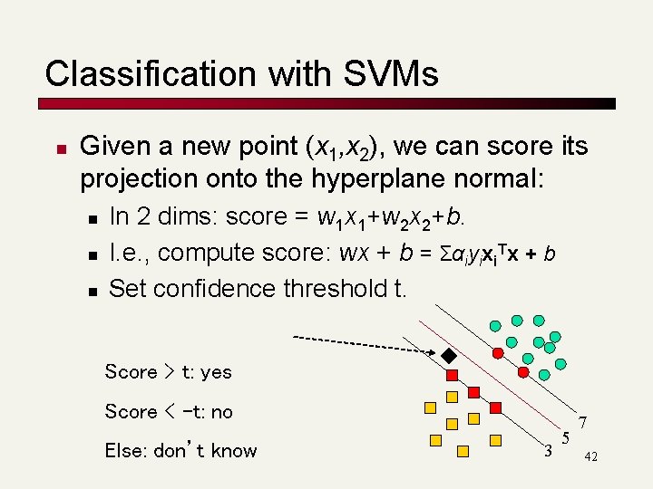
Classification with SVMs n Given a new point (x 1, x 2), we can score its projection onto the hyperplane normal: n n n In 2 dims: score = w 1 x 1+w 2 x 2+b. I. e. , compute score: wx + b = Σαiyixi. Tx + b Set confidence threshold t. Score > t: yes Score < -t: no Else: don’t know 3 5 7 42

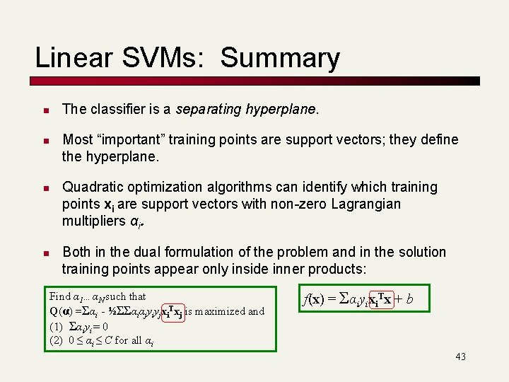
Linear SVMs: Summary n n The classifier is a separating hyperplane. Most “important” training points are support vectors; they define the hyperplane. Quadratic optimization algorithms can identify which training points xi are support vectors with non-zero Lagrangian multipliers αi. Both in the dual formulation of the problem and in the solution training points appear only inside inner products: Find α 1…αN such that Q(α) =Σαi - ½ΣΣαiαjyiyjxi. Txj is maximized and (1) Σαiyi = 0 (2) 0 ≤ αi ≤ C for all αi f(x) = Σαiyixi. Tx + b 43

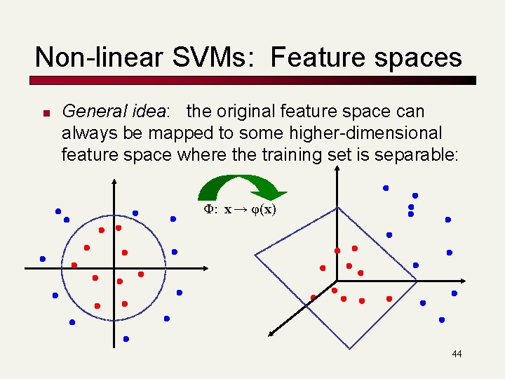
Non-linear SVMs: Feature spaces n General idea: the original feature space can always be mapped to some higher-dimensional feature space where the training set is separable: Φ: x → φ(x) 44

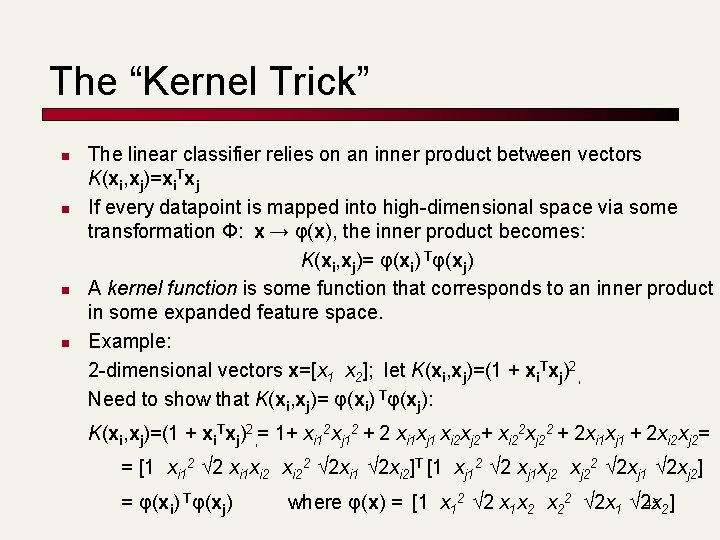
The “Kernel Trick” n n The linear classifier relies on an inner product between vectors K(xi, xj)=xi. Txj If every datapoint is mapped into high-dimensional space via some transformation Φ: x → φ(x), the inner product becomes: K(xi, xj)= φ(xi) Tφ(xj) A kernel function is some function that corresponds to an inner product in some expanded feature space. Example: 2 -dimensional vectors x=[x 1 x 2]; let K(xi, xj)=(1 + xi. Txj)2, Need to show that K(xi, xj)= φ(xi) Tφ(xj): K(xi, xj)=(1 + xi. Txj)2, = 1+ xi 12 xj 12 + 2 xi 1 xj 1 xi 2 xj 2+ xi 22 xj 22 + 2 xi 1 xj 1 + 2 xi 2 xj 2= = [1 xi 12 √ 2 xi 1 xi 22 √ 2 xi 1 √ 2 xi 2]T [1 xj 12 √ 2 xj 1 xj 22 √ 2 xj 1 √ 2 xj 2] = φ(xi) Tφ(xj) where φ(x) = [1 x 12 √ 2 x 1 x 2 x 22 √ 2 x 1 √ 2 x 45 2]

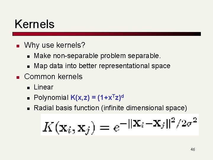
Kernels n Why use kernels? n n n Make non-separable problem separable. Map data into better representational space Common kernels n n n Linear Polynomial K(x, z) = (1+x. Tz)d Radial basis function (infinite dimensional space) 46