Classification Classification and regression What is classification What

Classification

Classification and regression What is classification? What is regression? p Classification by decision tree induction p Bayesian Classification p Other Classification Methods p n n Rule based K-NN SVM Bagging/Boosting

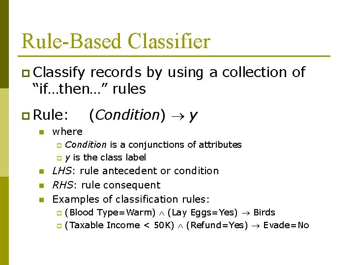
Rule-Based Classifier p Classify records by using a collection of “if…then…” rules p Rule: n where p p n n n (Condition) y Condition is a conjunctions of attributes y is the class label LHS: rule antecedent or condition RHS: rule consequent Examples of classification rules: p p (Blood Type=Warm) (Lay Eggs=Yes) Birds (Taxable Income < 50 K) (Refund=Yes) Evade=No

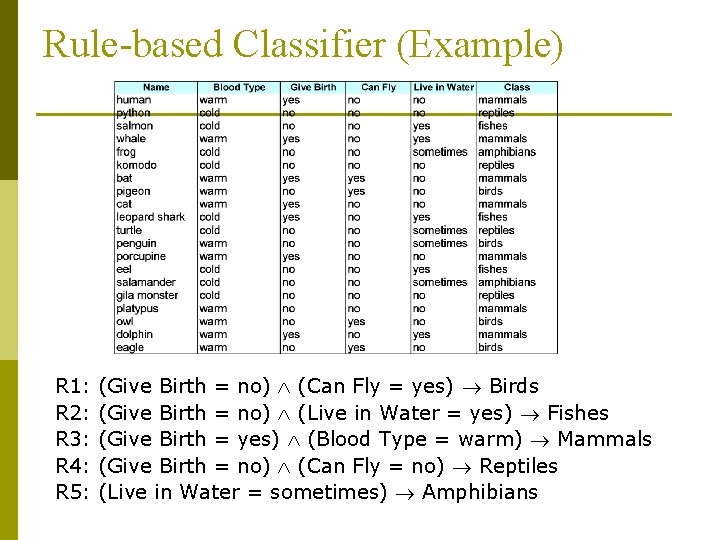
Rule-based Classifier (Example) R 1: R 2: R 3: R 4: R 5: (Give Birth = no) (Can Fly = yes) Birds (Give Birth = no) (Live in Water = yes) Fishes (Give Birth = yes) (Blood Type = warm) Mammals (Give Birth = no) (Can Fly = no) Reptiles (Live in Water = sometimes) Amphibians

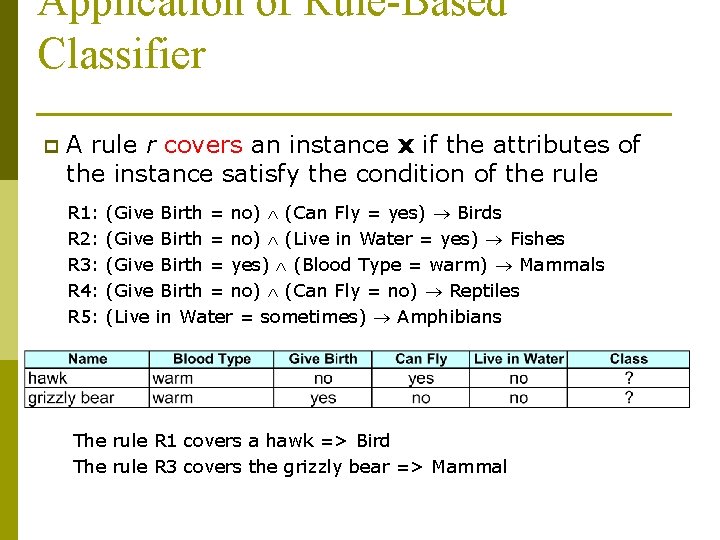
Application of Rule-Based Classifier p A rule r covers an instance x if the attributes of the instance satisfy the condition of the rule R 1: R 2: R 3: R 4: R 5: (Give Birth = no) (Can Fly = yes) Birds (Give Birth = no) (Live in Water = yes) Fishes (Give Birth = yes) (Blood Type = warm) Mammals (Give Birth = no) (Can Fly = no) Reptiles (Live in Water = sometimes) Amphibians The rule R 1 covers a hawk => Bird The rule R 3 covers the grizzly bear => Mammal

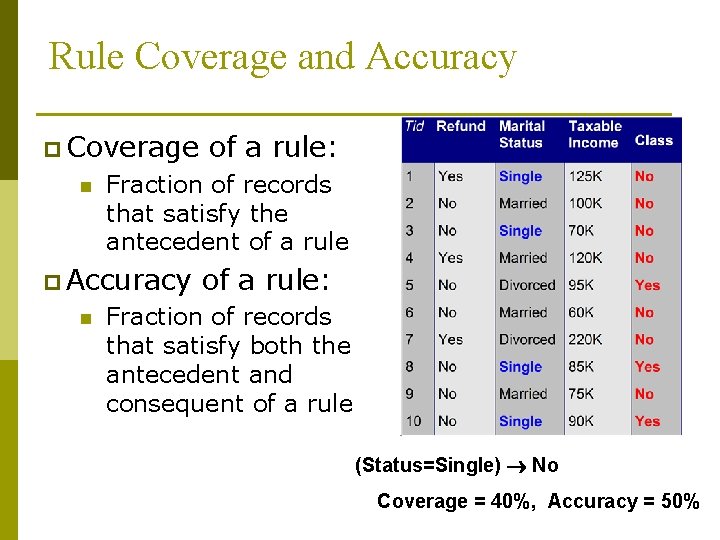
Rule Coverage and Accuracy p Coverage n Fraction of records that satisfy the antecedent of a rule p Accuracy n of a rule: Fraction of records that satisfy both the antecedent and consequent of a rule (Status=Single) No Coverage = 40%, Accuracy = 50%

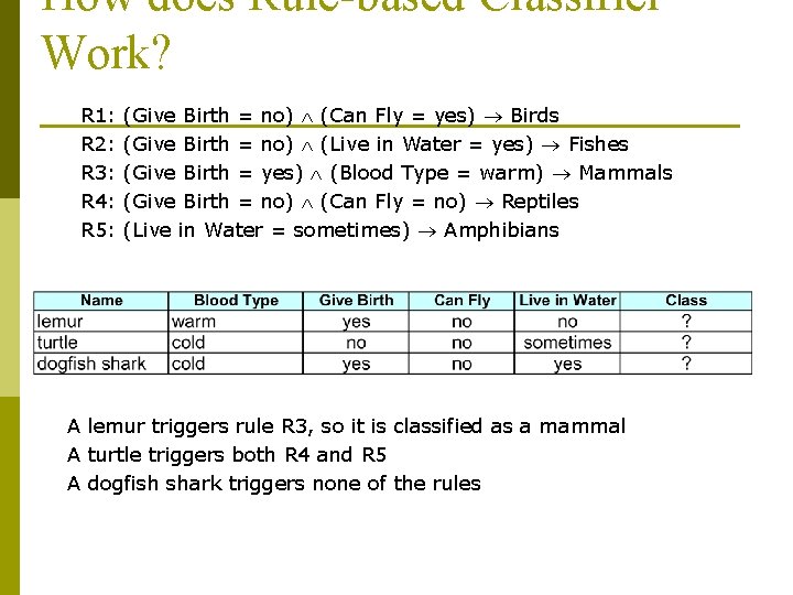
How does Rule-based Classifier Work? R 1: R 2: R 3: R 4: R 5: (Give Birth = no) (Can Fly = yes) Birds (Give Birth = no) (Live in Water = yes) Fishes (Give Birth = yes) (Blood Type = warm) Mammals (Give Birth = no) (Can Fly = no) Reptiles (Live in Water = sometimes) Amphibians A lemur triggers rule R 3, so it is classified as a mammal A turtle triggers both R 4 and R 5 A dogfish shark triggers none of the rules

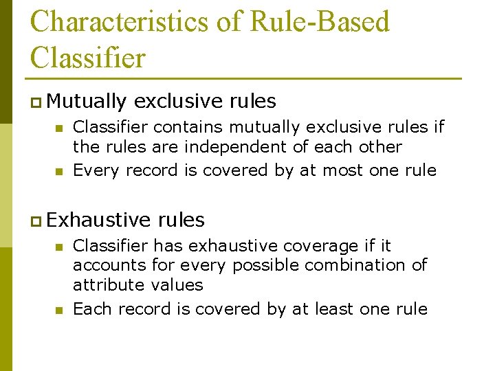
Characteristics of Rule-Based Classifier p Mutually n n exclusive rules Classifier contains mutually exclusive rules if the rules are independent of each other Every record is covered by at most one rule p Exhaustive n n rules Classifier has exhaustive coverage if it accounts for every possible combination of attribute values Each record is covered by at least one rule

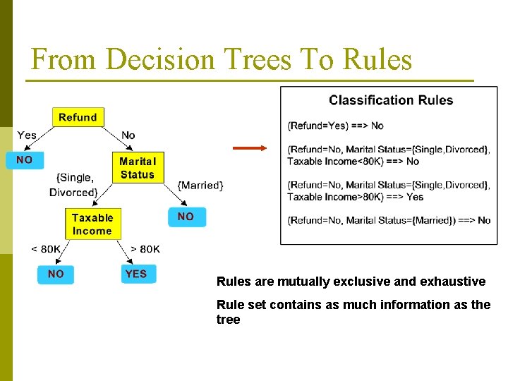
From Decision Trees To Rules are mutually exclusive and exhaustive Rule set contains as much information as the tree

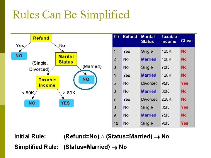
Rules Can Be Simplified Initial Rule: (Refund=No) (Status=Married) No Simplified Rule: (Status=Married) No

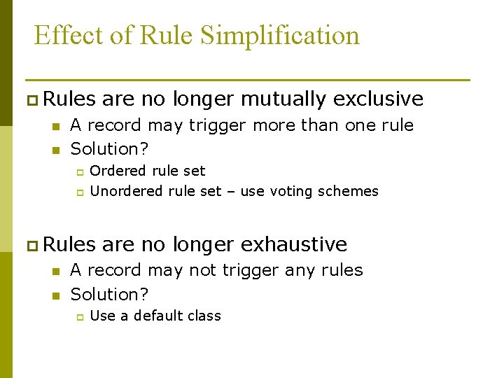
Effect of Rule Simplification p Rules n n A record may trigger more than one rule Solution? p p Ordered rule set Unordered rule set – use voting schemes p Rules n n are no longer mutually exclusive are no longer exhaustive A record may not trigger any rules Solution? p Use a default class

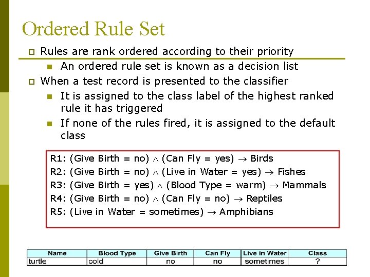
Ordered Rule Set p p Rules are rank ordered according to their priority n An ordered rule set is known as a decision list When a test record is presented to the classifier n It is assigned to the class label of the highest ranked rule it has triggered n If none of the rules fired, it is assigned to the default class R 1: R 2: R 3: R 4: R 5: (Give Birth = no) (Can Fly = yes) Birds (Give Birth = no) (Live in Water = yes) Fishes (Give Birth = yes) (Blood Type = warm) Mammals (Give Birth = no) (Can Fly = no) Reptiles (Live in Water = sometimes) Amphibians

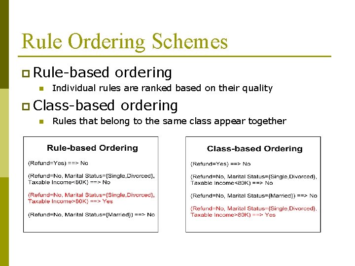
Rule Ordering Schemes p Rule-based n ordering Individual rules are ranked based on their quality p Class-based n ordering Rules that belong to the same class appear together

Building Classification Rules p Direct p p Method: Extract rules directly from data e. g. : RIPPER, CN 2, Holte’s 1 R p Indirect p p Method: Extract rules from other classification models (e. g. decision trees, etc). e. g: C 4. 5 rules

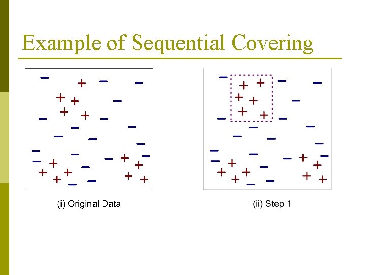
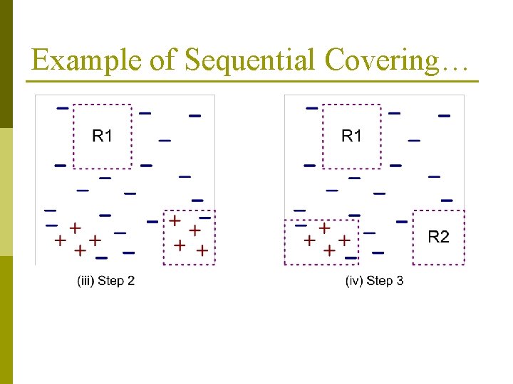
Direct Method: Sequential Covering 1. 2. 3. 4. Start from an empty rule Grow a rule using the Learn-One-Rule function Remove training records covered by the rule Repeat Step (2) and (3) until stopping criterion is met

Example of Sequential Covering

Example of Sequential Covering…

Aspects of Sequential Covering p Rule Growing p Instance p Rule Evaluation p Stopping p Rule Elimination Criterion Pruning

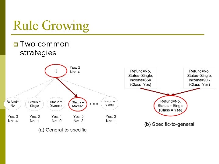
Rule Growing p Two common strategies

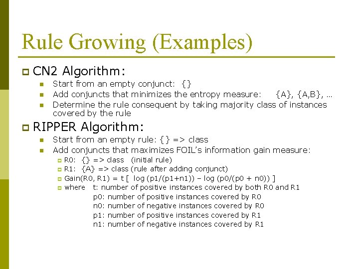
Rule Growing (Examples) p CN 2 Algorithm: n n n p Start from an empty conjunct: {} Add conjuncts that minimizes the entropy measure: {A}, {A, B}, … Determine the rule consequent by taking majority class of instances covered by the rule RIPPER Algorithm: n n Start from an empty rule: {} => class Add conjuncts that maximizes FOIL’s information gain measure: p p R 0: {} => class (initial rule) R 1: {A} => class (rule after adding conjunct) Gain(R 0, R 1) = t [ log (p 1/(p 1+n 1)) – log (p 0/(p 0 + n 0)) ] where t: number of positive instances covered by both R 0 and R 1 p 0: number of positive instances covered by R 0 n 0: number of negative instances covered by R 0 p 1: number of positive instances covered by R 1 n 1: number of negative instances covered by R 1

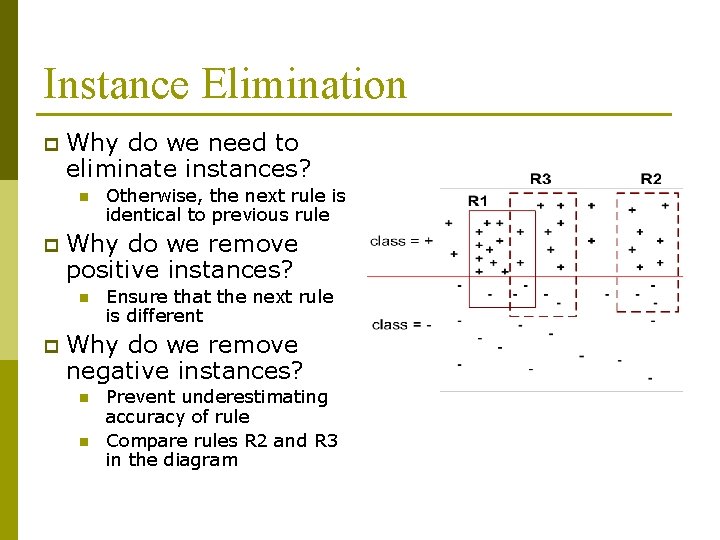
Instance Elimination p Why do we need to eliminate instances? n p Why do we remove positive instances? n p Otherwise, the next rule is identical to previous rule Ensure that the next rule is different Why do we remove negative instances? n n Prevent underestimating accuracy of rule Compare rules R 2 and R 3 in the diagram

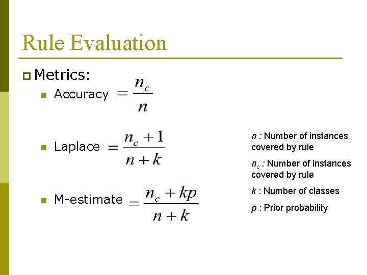
Rule Evaluation p Metrics: n n Accuracy Laplace n : Number of instances covered by rule nc : Number of instances covered by rule n M-estimate k : Number of classes p : Prior probability

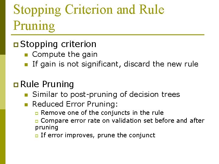
Stopping Criterion and Rule Pruning p Stopping n n Compute the gain If gain is not significant, discard the new rule p Rule n n criterion Pruning Similar to post-pruning of decision trees Reduced Error Pruning: Remove one of the conjuncts in the rule p Compare error rate on validation set before and after pruning p If error improves, prune the conjunct p

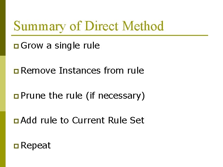
Summary of Direct Method p Grow a single rule p Remove p Prune p Add Instances from rule the rule (if necessary) rule to Current Rule Set p Repeat

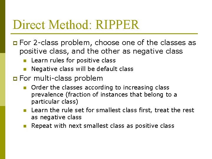
Direct Method: RIPPER p For 2 -class problem, choose one of the classes as positive class, and the other as negative class n n p Learn rules for positive class Negative class will be default class For multi-class problem n n n Order the classes according to increasing class prevalence (fraction of instances that belong to a particular class) Learn the rule set for smallest class first, treat the rest as negative class Repeat with next smallest class as positive class

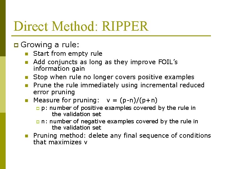
Direct Method: RIPPER p Growing a rule: n n n Start from empty rule Add conjuncts as long as they improve FOIL’s information gain Stop when rule no longer covers positive examples Prune the rule immediately using incremental reduced error pruning Measure for pruning: v = (p-n)/(p+n) p p n p: number of positive examples covered by the rule in the validation set n: number of negative examples covered by the rule in the validation set Pruning method: delete any final sequence of conditions that maximizes v

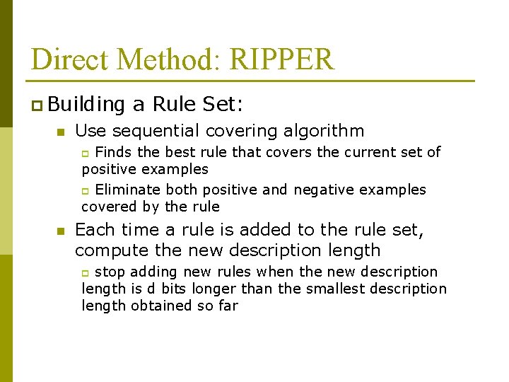
Direct Method: RIPPER p Building n a Rule Set: Use sequential covering algorithm Finds the best rule that covers the current set of positive examples p Eliminate both positive and negative examples covered by the rule p n Each time a rule is added to the rule set, compute the new description length stop adding new rules when the new description length is d bits longer than the smallest description length obtained so far p

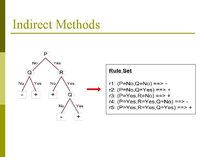
Indirect Methods

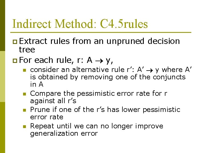
Indirect Method: C 4. 5 rules p Extract rules from an unpruned decision tree p For each rule, r: A y, n n consider an alternative rule r’: A’ y where A’ is obtained by removing one of the conjuncts in A Compare the pessimistic error rate for r against all r’s Prune if one of the r’s has lower pessimistic error rate Repeat until we can no longer improve generalization error

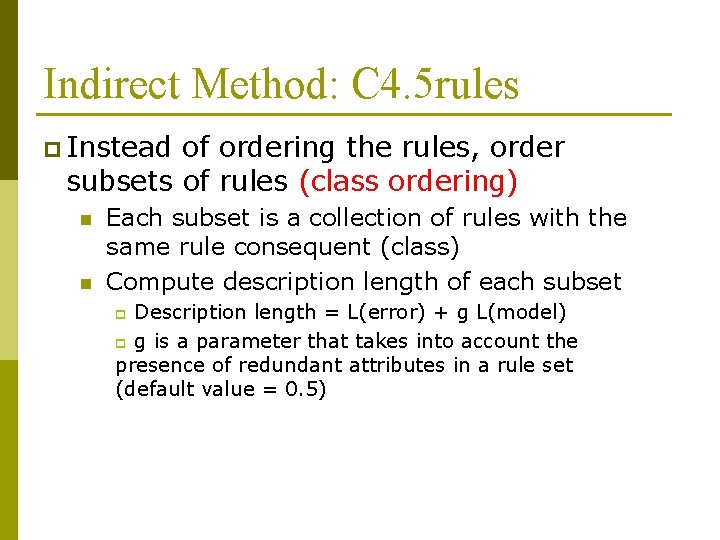
Indirect Method: C 4. 5 rules p Instead of ordering the rules, order subsets of rules (class ordering) n n Each subset is a collection of rules with the same rule consequent (class) Compute description length of each subset Description length = L(error) + g L(model) p g is a parameter that takes into account the presence of redundant attributes in a rule set (default value = 0. 5) p

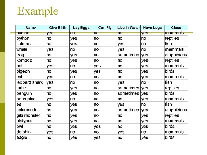
Example

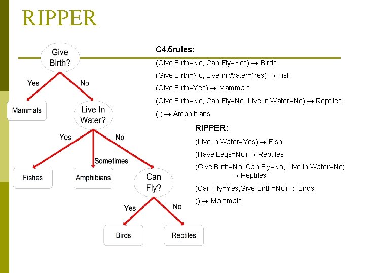
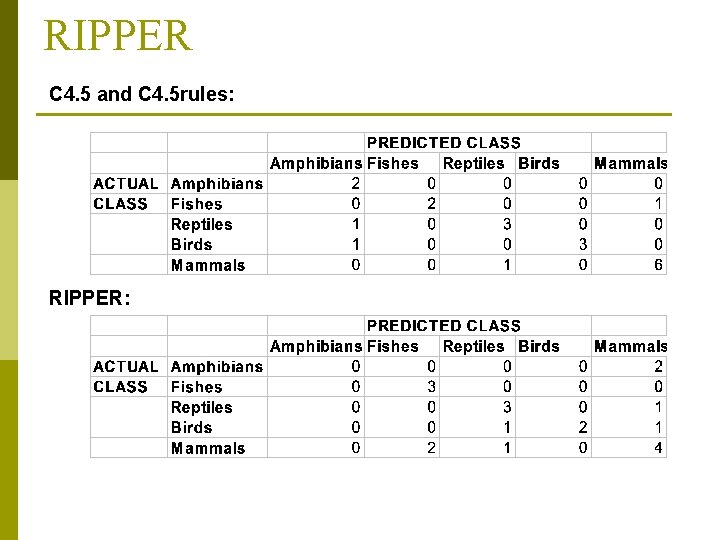
RIPPER C 4. 5 rules: (Give Birth=No, Can Fly=Yes) Birds (Give Birth=No, Live in Water=Yes) Fish (Give Birth=Yes) Mammals (Give Birth=No, Can Fly=No, Live in Water=No) Reptiles ( ) Amphibians RIPPER: (Live in Water=Yes) Fish (Have Legs=No) Reptiles (Give Birth=No, Can Fly=No, Live In Water=No) Reptiles (Can Fly=Yes, Give Birth=No) Birds () Mammals

RIPPER C 4. 5 and C 4. 5 rules: RIPPER:

Advantages of Rule-Based Classifiers p As highly expressive as decision trees p Easy to interpret p Easy to generate p Can classify new instances rapidly p Performance comparable to decision trees

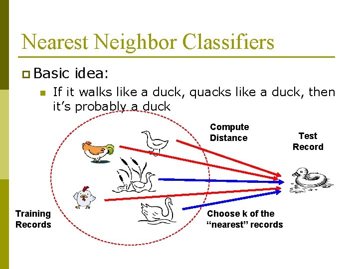
Nearest Neighbor Classifiers p Basic n idea: If it walks like a duck, quacks like a duck, then it’s probably a duck Compute Distance Training Records Choose k of the “nearest” records Test Record

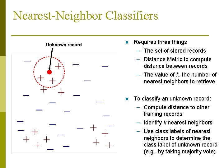
Nearest-Neighbor Classifiers l Requires three things – The set of stored records – Distance Metric to compute distance between records – The value of k, the number of nearest neighbors to retrieve l To classify an unknown record: – Compute distance to other training records – Identify k nearest neighbors – Use class labels of nearest neighbors to determine the class label of unknown record (e. g. , by taking majority vote)

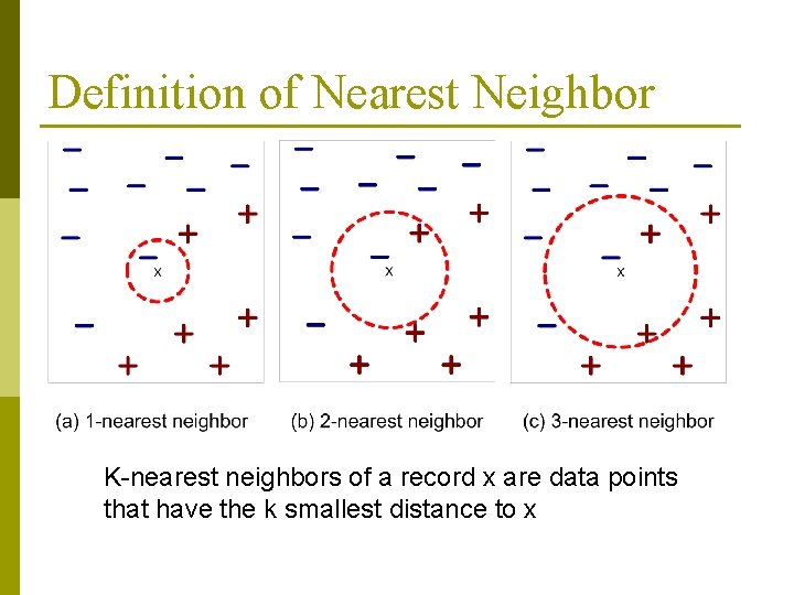
Definition of Nearest Neighbor K-nearest neighbors of a record x are data points that have the k smallest distance to x

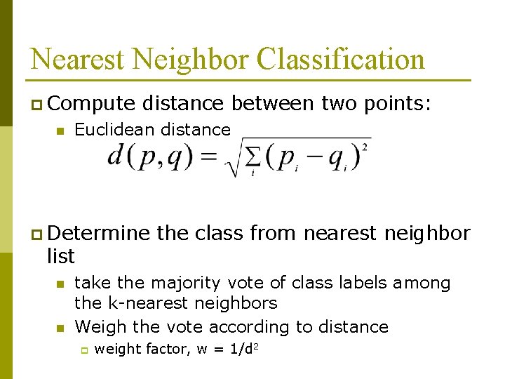
Nearest Neighbor Classification p Compute n distance between two points: Euclidean distance p Determine list n n the class from nearest neighbor take the majority vote of class labels among the k-nearest neighbors Weigh the vote according to distance p weight factor, w = 1/d 2

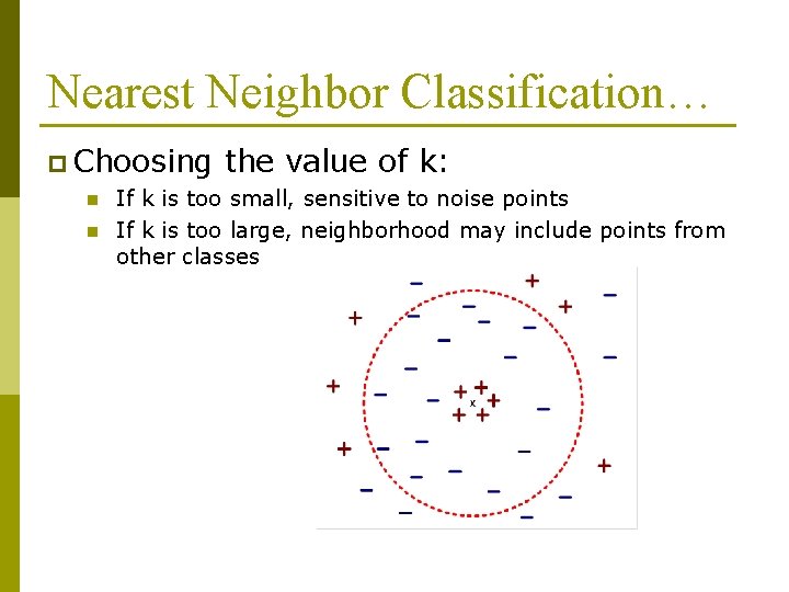
Nearest Neighbor Classification… p Choosing n n the value of k: If k is too small, sensitive to noise points If k is too large, neighborhood may include points from other classes

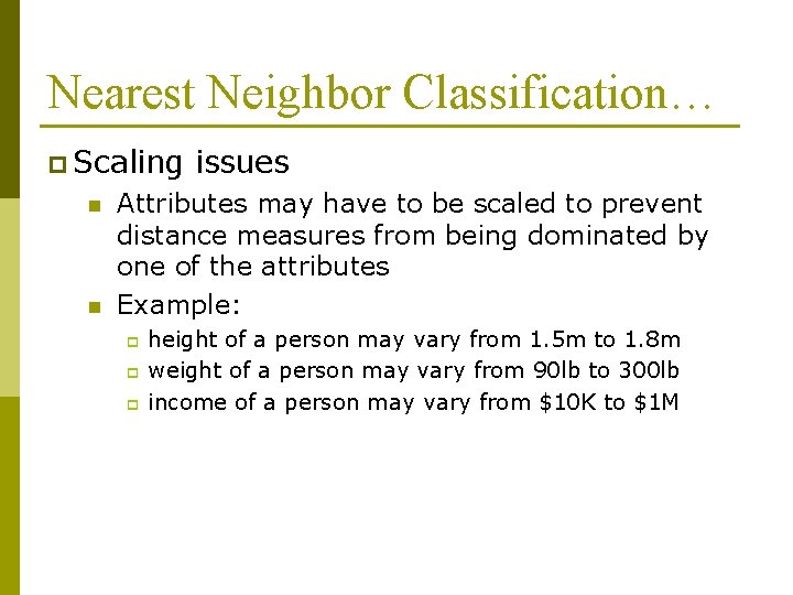
Nearest Neighbor Classification… p Scaling n n issues Attributes may have to be scaled to prevent distance measures from being dominated by one of the attributes Example: p p p height of a person may vary from 1. 5 m to 1. 8 m weight of a person may vary from 90 lb to 300 lb income of a person may vary from $10 K to $1 M

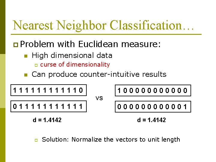
Nearest Neighbor Classification… p Problem n High dimensional data p n with Euclidean measure: curse of dimensionality Can produce counter-intuitive results 1111110 vs 1000000 0111111 0000001 d = 1. 4142 p Solution: Normalize the vectors to unit length

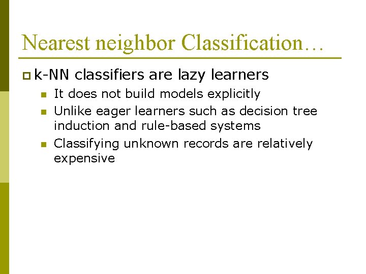
Nearest neighbor Classification… p k-NN n n n classifiers are lazy learners It does not build models explicitly Unlike eager learners such as decision tree induction and rule-based systems Classifying unknown records are relatively expensive

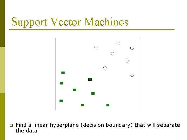
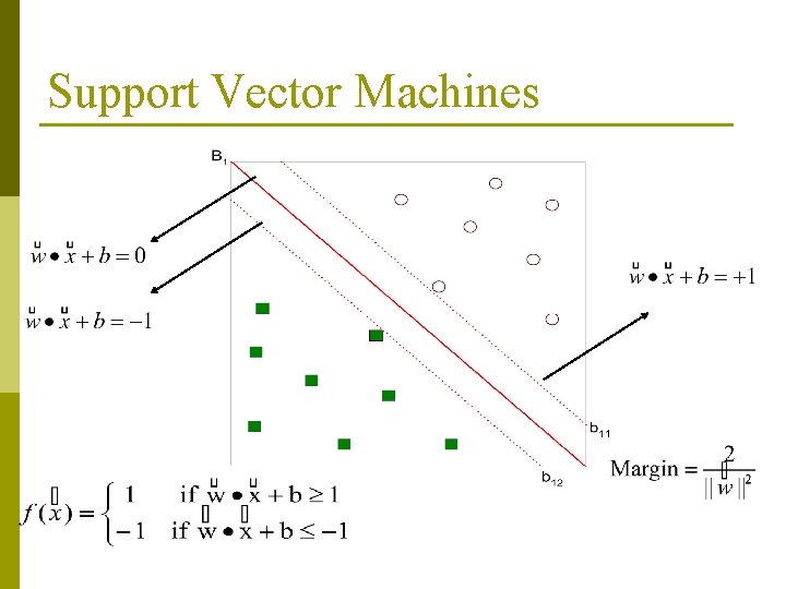
Support Vector Machines p Find a linear hyperplane (decision boundary) that will separate the data

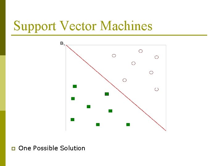
Support Vector Machines p One Possible Solution

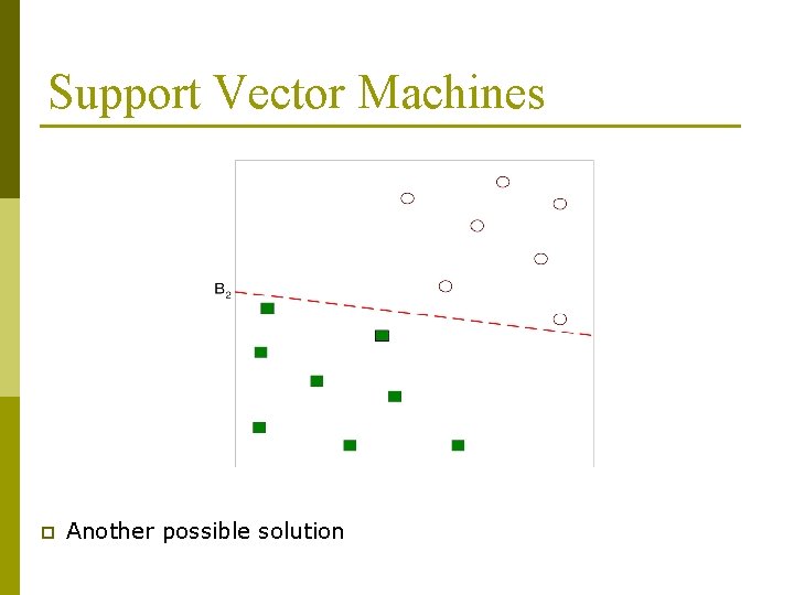
Support Vector Machines p Another possible solution

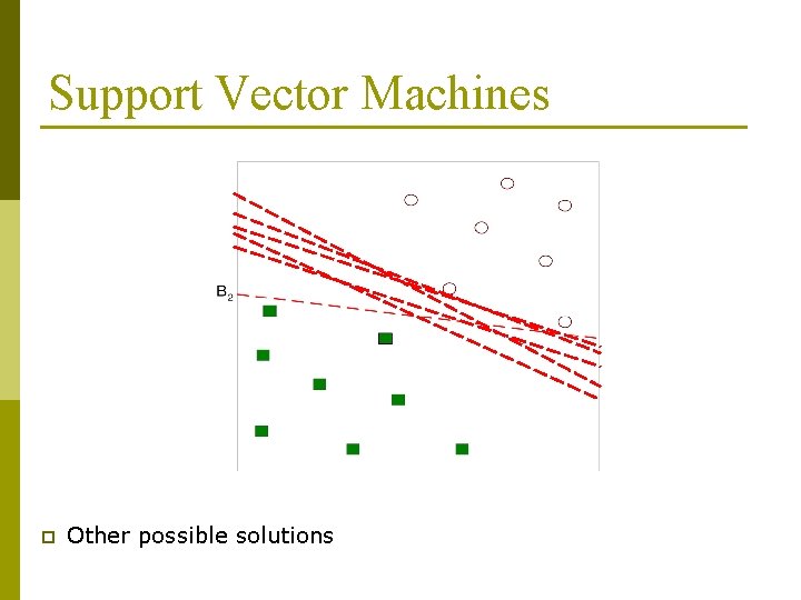
Support Vector Machines p Other possible solutions

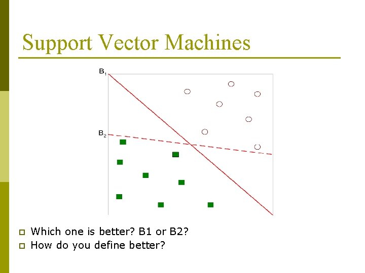
Support Vector Machines p p Which one is better? B 1 or B 2? How do you define better?

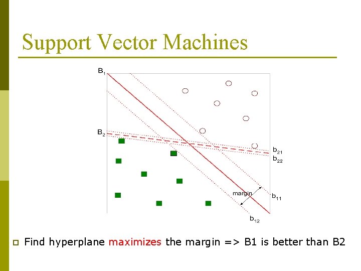
Support Vector Machines p Find hyperplane maximizes the margin => B 1 is better than B 2

Support Vector Machines

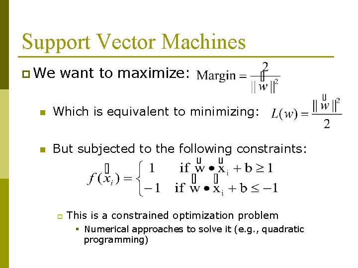
Support Vector Machines p We want to maximize: n Which is equivalent to minimizing: n But subjected to the following constraints: p This is a constrained optimization problem § Numerical approaches to solve it (e. g. , quadratic programming)

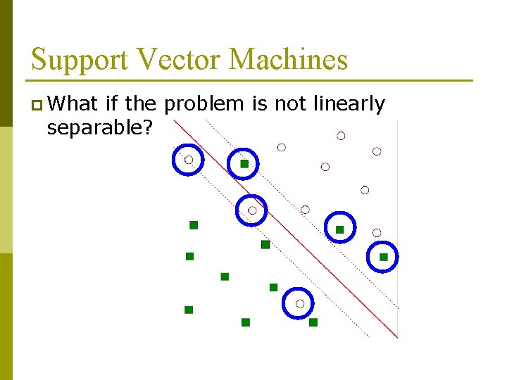
Support Vector Machines p What if the problem is not linearly separable?

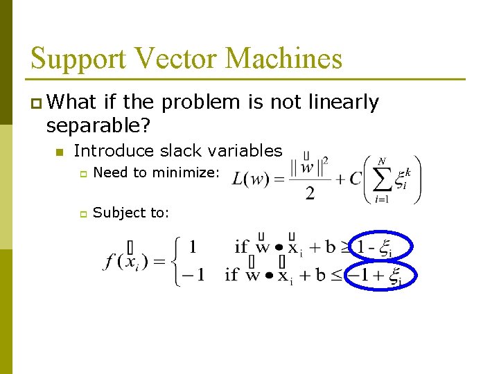
Support Vector Machines p What if the problem is not linearly separable? n Introduce slack variables p Need to minimize: p Subject to:

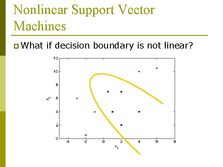
Nonlinear Support Vector Machines p What if decision boundary is not linear?

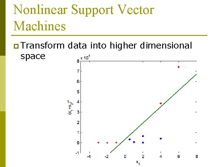
Nonlinear Support Vector Machines p Transform space data into higher dimensional

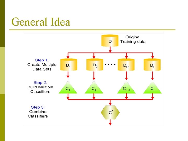
Ensemble Methods p Construct a set of classifiers from the training data p Predict class label of previously unseen records by aggregating predictions made by multiple classifiers

General Idea

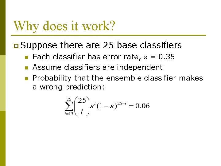
Why does it work? p Suppose n n n there are 25 base classifiers Each classifier has error rate, = 0. 35 Assume classifiers are independent Probability that the ensemble classifier makes a wrong prediction:

Examples of Ensemble Methods p How to generate an ensemble of classifiers? n Bagging n Boosting

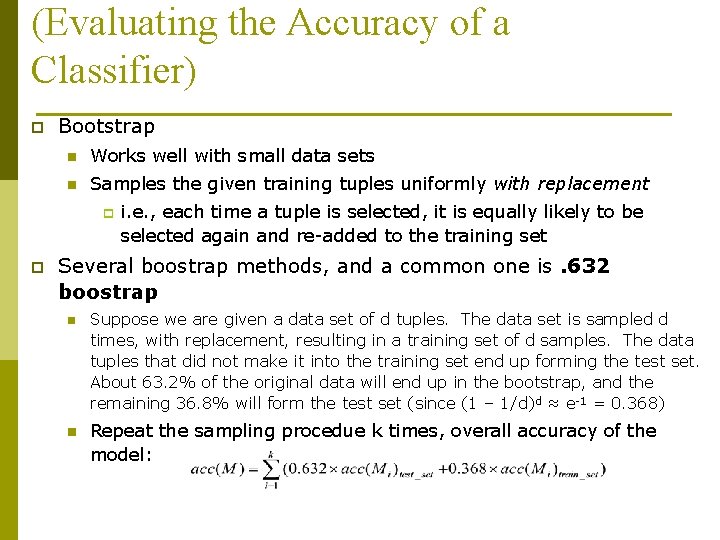
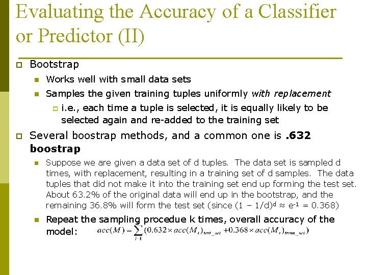
(Evaluating the Accuracy of a Classifier) p Bootstrap n Works well with small data sets n Samples the given training tuples uniformly with replacement p p i. e. , each time a tuple is selected, it is equally likely to be selected again and re-added to the training set Several boostrap methods, and a common one is. 632 boostrap n Suppose we are given a data set of d tuples. The data set is sampled d times, with replacement, resulting in a training set of d samples. The data tuples that did not make it into the training set end up forming the test set. About 63. 2% of the original data will end up in the bootstrap, and the remaining 36. 8% will form the test set (since (1 – 1/d)d ≈ e-1 = 0. 368) n Repeat the sampling procedue k times, overall accuracy of the model:

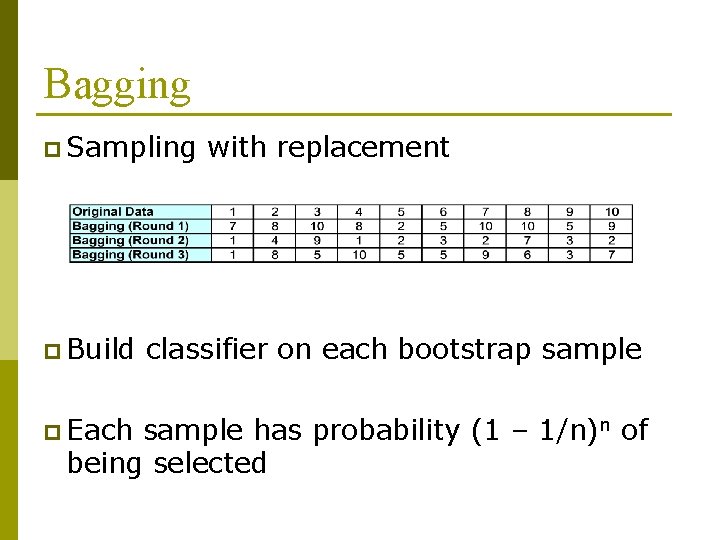
Bagging p Sampling p Build p Each with replacement classifier on each bootstrap sample has probability (1 – 1/n)n of being selected

Boosting p An iterative procedure to adaptively change distribution of training data by focusing more on previously misclassified records n n Initially, all N records are assigned equal weights Unlike bagging, weights may change at the end of boosting round

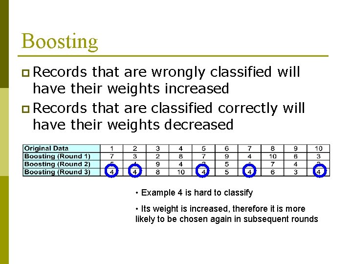
Boosting p Records that are wrongly classified will have their weights increased p Records that are classified correctly will have their weights decreased • Example 4 is hard to classify • Its weight is increased, therefore it is more likely to be chosen again in subsequent rounds

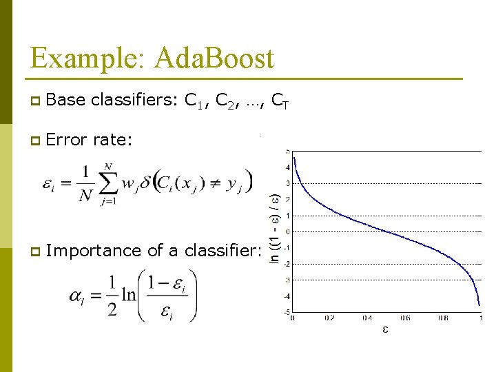
Example: Ada. Boost p Base classifiers: C 1, C 2, …, CT p Error rate: p Importance of a classifier:

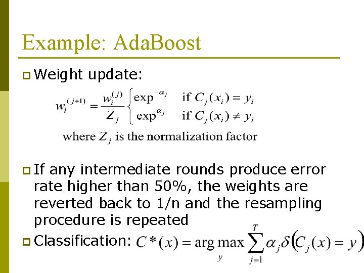
Example: Ada. Boost p Weight p If update: any intermediate rounds produce error rate higher than 50%, the weights are reverted back to 1/n and the resampling procedure is repeated p Classification:

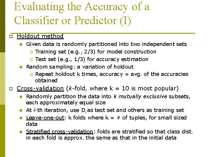
Evaluating the Accuracy of a Classifier or Predictor (I) p Holdout method n n p Given data is randomly partitioned into two independent sets p Training set (e. g. , 2/3) for model construction p Test set (e. g. , 1/3) for accuracy estimation Random sampling: a variation of holdout p Repeat holdout k times, accuracy = avg. of the accuracies obtained Cross-validation (k-fold, where k = 10 is most popular) n n Randomly partition the data into k mutually exclusive subsets, each approximately equal size At i-th iteration, use Di as test set and others as training set Leave-one-out: k folds where k = # of tuples, for small sized data Stratified cross-validation: folds are stratified so that class dist. in each fold is approx. the same as that in the initial data

Evaluating the Accuracy of a Classifier or Predictor (II) p Bootstrap n Works well with small data sets n Samples the given training tuples uniformly with replacement p p i. e. , each time a tuple is selected, it is equally likely to be selected again and re-added to the training set Several boostrap methods, and a common one is. 632 boostrap n Suppose we are given a data set of d tuples. The data set is sampled d times, with replacement, resulting in a training set of d samples. The data tuples that did not make it into the training set end up forming the test set. About 63. 2% of the original data will end up in the bootstrap, and the remaining 36. 8% will form the test set (since (1 – 1/d)d ≈ e-1 = 0. 368) n Repeat the sampling procedue k times, overall accuracy of the model:

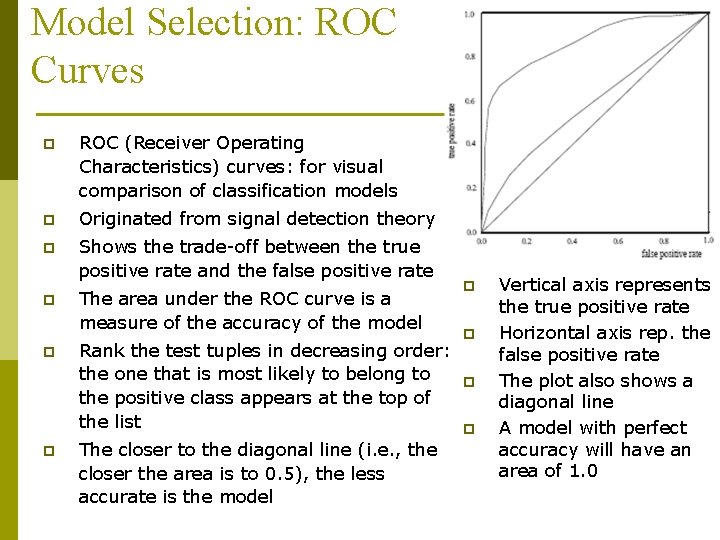
Model Selection: ROC Curves p ROC (Receiver Operating Characteristics) curves: for visual comparison of classification models p Originated from signal detection theory p Shows the trade-off between the true positive rate and the false positive rate p p p The area under the ROC curve is a measure of the accuracy of the model Rank the test tuples in decreasing order: the one that is most likely to belong to the positive class appears at the top of the list The closer to the diagonal line (i. e. , the closer the area is to 0. 5), the less accurate is the model p p Vertical axis represents the true positive rate Horizontal axis rep. the false positive rate The plot also shows a diagonal line A model with perfect accuracy will have an area of 1. 0