Classification Bayesian Classifiers Jeff Howbert Introduction to Machine

Classification Bayesian Classifiers Jeff Howbert Introduction to Machine Learning Winter 2014 1

Bayesian classification l A probabilistic framework for solving classification problems. – Used where class assignment is not deterministic, i. e. a particular set of attribute values will sometimes be associated with one class, sometimes with another. – Requires estimation of posterior probability for each class, given a set of attribute values: for each class Ci – Then use decision theory to make predictions for a new sample x Jeff Howbert Introduction to Machine Learning Winter 2014 2

Bayesian classification l l Conditional probability: Bayes theorem: posterior probability Jeff Howbert likelihood prior probability evidence Introduction to Machine Learning Winter 2014 3

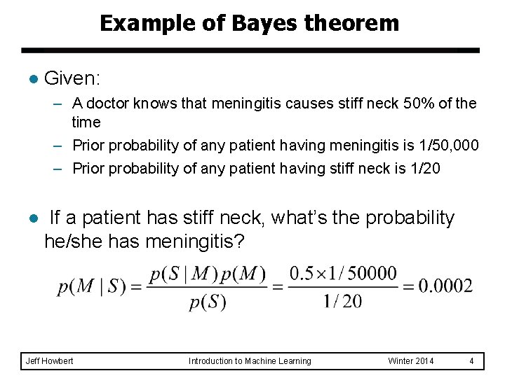
Example of Bayes theorem l Given: – A doctor knows that meningitis causes stiff neck 50% of the time – Prior probability of any patient having meningitis is 1/50, 000 – Prior probability of any patient having stiff neck is 1/20 l If a patient has stiff neck, what’s the probability he/she has meningitis? Jeff Howbert Introduction to Machine Learning Winter 2014 4

Bayesian classifiers l Treat each attribute and class label as random variables. l Given a sample x with attributes ( x 1, x 2, … , xn ): – Goal is to predict class C. – Specifically, we want to find the value of Ci that maximizes p( Ci | x 1, x 2, … , xn ). l Can we estimate p( Ci | x 1, x 2, … , xn ) directly from data? Jeff Howbert Introduction to Machine Learning Winter 2014 5

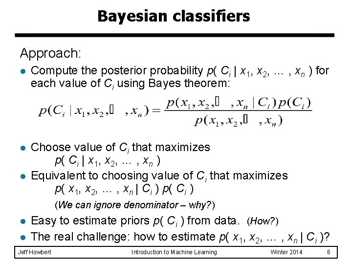
Bayesian classifiers Approach: l Compute the posterior probability p( Ci | x 1, x 2, … , xn ) for each value of Ci using Bayes theorem: l Choose value of Ci that maximizes p( Ci | x 1, x 2, … , xn ) Equivalent to choosing value of Ci that maximizes p( x 1, x 2, … , xn | Ci ) p( Ci ) l (We can ignore denominator – why? ) l l Easy to estimate priors p( Ci ) from data. (How? ) The real challenge: how to estimate p( x 1, x 2, … , xn | Ci )? Jeff Howbert Introduction to Machine Learning Winter 2014 6

Bayesian classifiers l How to estimate p( x 1, x 2, … , xn | Ci )? l In the general case, where the attributes xj have dependencies, this requires estimating the full joint distribution p( x 1, x 2, … , xn ) for each class Ci. l There is almost never enough data to confidently make such estimates. Jeff Howbert Introduction to Machine Learning Winter 2014 7

Naïve Bayes classifier l Assume independence among attributes xj when class is given: p( x 1, x 2, … , xn | Ci ) = p( x 1 | Ci ) p( x 2 | Ci ) … p( xn | Ci ) l Usually straightforward and practical to estimate p( xj | Ci ) for all xj and Ci. l New sample is classified to Ci if p( Ci ) p( xj | Ci ) is maximal. Jeff Howbert Introduction to Machine Learning Winter 2014 8

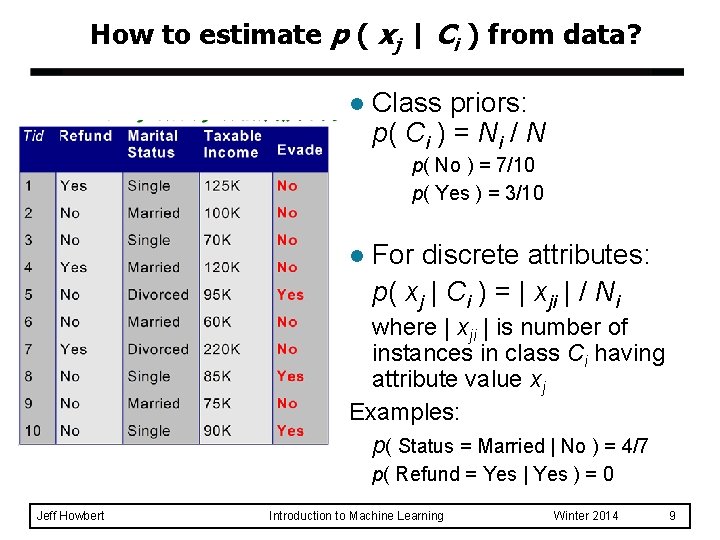
How to estimate p ( xj | Ci ) from data? l Class priors: p( Ci ) = Ni / N p( No ) = 7/10 p( Yes ) = 3/10 l For discrete attributes: p( xj | Ci ) = | xji | / Ni where | xji | is number of instances in class Ci having attribute value xj Examples: p( Status = Married | No ) = 4/7 p( Refund = Yes | Yes ) = 0 Jeff Howbert Introduction to Machine Learning Winter 2014 9

How to estimate p ( xj | Ci ) from data? l For continuous attributes: – Discretize the range into bins u replace with an ordinal attribute – Two-way split: ( xi < v ) or ( xi > v ) u replace with a binary attribute – Probability density estimation: assume attribute follows some standard parametric probability distribution (usually a Gaussian) u use data to estimate parameters of distribution (e. g. mean and variance) u once distribution is known, can use it to estimate the conditional probability p( xj | Ci ) u Jeff Howbert Introduction to Machine Learning Winter 2014 10

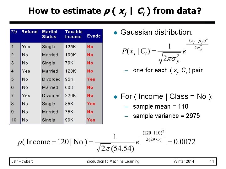
How to estimate p ( xj | Ci ) from data? l Gaussian distribution: – one for each ( xj, Ci ) pair l For ( Income | Class = No ): – sample mean = 110 – sample variance = 2975 Jeff Howbert Introduction to Machine Learning Winter 2014 11

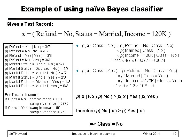
Example of using naïve Bayes classifier Given a Test Record: p( Refund = Yes | No ) = 3/7 p( Refund = No | No ) = 4/7 p( Refund = Yes | Yes ) = 0/3 p( Refund = No | Yes ) = 3/3 p( Marital Status = Single | No ) = 2/7 p( Marital Status = Divorced | No ) = 1/7 p( Marital Status = Married | No ) = 4/7 p( Marital Status = Single | Yes ) = 2/3 p( Marital Status = Divorced | Yes ) = 1/3 p( Marital Status = Married | Yes ) = 0/3 l p( x | Class = No ) = p( Refund = No | Class = No) p( Married | Class = No ) p( Income = 120 K | Class = No ) = 4/7 0. 0072 = 0. 0024 l p( x | Class = Yes ) = p( Refund = No | Class = Yes) p( Married | Class = Yes ) p( Income = 120 K | Class = Yes ) = 1 0 1. 2 10 -9 = 0 For Taxable Income: If Class = No: sample mean = 110 sample variance = 2975 If Class = Yes: sample mean = 90 sample variance = 25 p( x | No ) p( No ) > p( x | Yes ) p( Yes ) therefore p( No | x ) > p( Yes | x ) => Class = No Jeff Howbert Introduction to Machine Learning Winter 2014 12

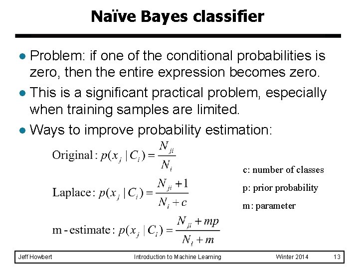
Naïve Bayes classifier Problem: if one of the conditional probabilities is zero, then the entire expression becomes zero. l This is a significant practical problem, especially when training samples are limited. l Ways to improve probability estimation: l c: number of classes p: prior probability m: parameter Jeff Howbert Introduction to Machine Learning Winter 2014 13

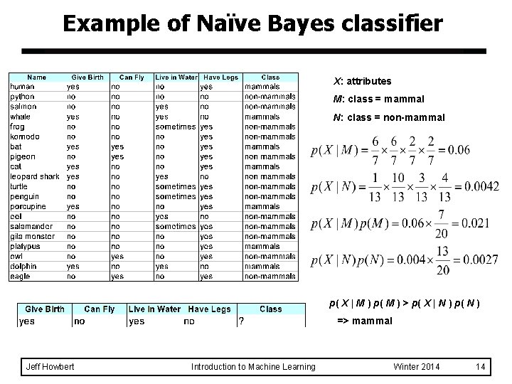
Example of Naïve Bayes classifier X: attributes M: class = mammal N: class = non-mammal p( X | M ) p( M ) > p( X | N ) p( N ) => mammal Jeff Howbert Introduction to Machine Learning Winter 2014 14

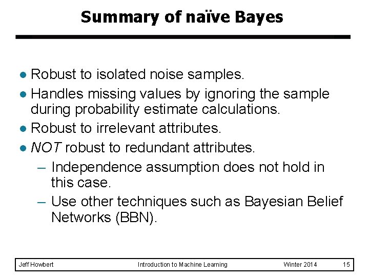
Summary of naïve Bayes Robust to isolated noise samples. l Handles missing values by ignoring the sample during probability estimate calculations. l Robust to irrelevant attributes. l NOT robust to redundant attributes. – Independence assumption does not hold in this case. – Use other techniques such as Bayesian Belief Networks (BBN). l Jeff Howbert Introduction to Machine Learning Winter 2014 15