Classification and Regression Trees CART and Random Forests

Classification and Regression Trees (CART) and Random Forests “Just as the ability to devise simple but evocative models is the signature of the great scientist so overelaboration and overparameterization is often the mark of mediocrity”- George E. P. Box, 1976

Machine Learning Methods • Completely different in flavor than parametric classical statistical inference • Often borrowing ideas from computer science and engineering where characterizing uncertainty is de-emphasized, more algorithmic than stochastic • Learn from the data as opposed to cast the data into a linear/structured model

Supervised Learning Setup • Output measurement Y (also called class label, response, dependent variable, target). • Vector of p input measurements X (also called predictors, regressors, covariates, independent variables, features). • Y takes values in a finite, unordered set (binary: alive / dead, continuous measure: blood lead). • We have training data (y 1, x 1), …. (yn, xn). These are observations (instances) of these measurements.

Objectives • On the basis of the training data we would like to – Accurately predict unseen test cases – Understand which inputs affect the output, and how – Assess the quality of our predictions and inferences

General Tree-based methods • Prediction, classification and assessment of variable importance are critical questions in statistical inference. • Recursive partitioning is a general strategy where the feature space (e. g. space spanned by all 20 predictor variables in NHANES) is split into regions containing observations with similar response values.

Classification vs Regression • Classification Tree: When Y (outcome) is binary/unordered categorical, you want to assign each subject to a category Y=k, Error assessment through misclassification cost. • Regression Tree: Y is continuous or ordered discrete values. Prediction error measured by squared or relative absolute difference between observed and predicted values.

Classification Tree: 3 class labels, two predictors, partition X space (feature space) into rectangular sets Loh et al, 2011

Regression Tree Prediction by group mean

Classification and Regression Trees • Breiman, Friedman, Olshen and Stone (1984), proposed this 30 years ago. • Feature space recursively partitioned into rectangular areas such that observations with similar responses are grouped together. • When you stop you provide a common prediction for Y for subjects in the same group.

What is the difference with linear regression? • Linear in predictors? • Multiple splits of the same predictor • Non-linear and even non-monotone associations are identified in data-adaptive way. • Interactions are allowed, but the focus is identification of association/variable importance, allowing for interactions.

Why use trees ? • yields relatively simple and easy to comprehend models. • frequently more accurate than parametric tools. • method can sift through any number of variables. • can separate relevant from irrelevant predictors.

1. Universally applicable to both classification and regression problems with no assumptions on the data structure. 2. Good properties: variable selection, missing data, mixed predictors. 3. Picture of the tree gives valuable insights into which variables are important and where. 4. Terminal groups suggest natural clustering of data into homogeneous groups.

CART Biomedical Applications • CART has had an enormous impact in biomedical studies • A large number of cancer and coronary heart disease studies published • Over 1000 publications using CART in last decade • Recently, a growing number of applications in other fields – Market research – Credit risk assessment – Financial markets

Why is CART receiving more attention ? • Availability of huge data sets requiring analysis • Need to automate or accelerate and improve analysis process • Rising interest in data mining • New software and documentation make techniques accessible to researchers • Next generation CART techniques appear to be even better than former

• Well illustrated with a famous example : the UCSD Heart Disease study • Given the diagnosis of a heart attack based on – Chest pain, Indicative EKGs, Elevation of enzymes typically released by damaged heart muscle • Predict who is at risk of a 2 nd heart attack and early death within 30 days – Prediction will determine treatment program (intensive care or not) • For each patient about 100 variables were available, including – demographics, medical history, lab results – 19 noninvasive variables were used in the analysis

2 nd Heart Attack Risk Tree • Example of a CLASSIFICATION tree • Dependent variable is binary (SURVIVE, DEATH) • Want to predict class membership • Trees with a continuous dependent variable are called REGRESSION trees

N = 215 <= 91 SURVIVE 178 82. 8% DEAD 37 17. 2% > 91 Is BP <= 91 ? SURVIVE 6 30% DEAD 14 70% <= 62. 5 NODE = DEAD N = 195 SURVIVE 172 88. 2% DEAD 23 11. 8% > 62. 5 AGE <= 62. 5 ? SURVIVE 102 98. 1% DEAD 2 1. 9% N = 91 YES NODE = SURVIVE 14 46. 6% DEAD 16 53. 4% NODE = DEAD SURVIVE 70 76. 9% DEAD 21 23. 1% Sinus Tachycardia ? NO SURVIVE 56 91. 8% DEAD 5 8. 2% NODE = SURVIVE

What’s new in this method ? • Entire tree represents a complete analysis or model • Has the form of a decision tree • Root of inverted tree contains all data • Root gives rise to child nodes which in turn can give rise to their own children

• At some point a given path ends in a terminal node • Terminal node classifies a subject • Terminal nodes associated with a single class – any case arriving at a terminal node is assigned to that class • Path through the tree governed by answers to QUESTIONS or RULES

Questions of the form: • Is continuous variable X c ? – reports a split value which is the mid-point between two actual data values: better for future data • Does categorical (nominal) variable D take on levels i, j, or k ? – e. g. Is geographic region 1, 2, 4, or 7 ? • Question is formulated so that only two answers possible – called binary partitioning – partitions can also be split into subpartitions : hence procedure is recursive

Accuracy of a Tree • For classification trees – all objects reaching a terminal node are classified in the same way • e. g. all heart attack victims with BP > 91 and AGE less than 62. 5 are classified as SURVIVORS – classification is same regardless of other medical history and lab results • Some cases may be misclassified – R(T) = % of learning sample misclassified in tree T – R(t) = % of learning sample in node t misclassified – T identifies a TREE – t identifies a NODE

Prediction Success Table CLASSIFIED AS TRUE Survive Dead Total Survive 158 20 178 Dead 7 30 37 Total 165 50 215 • % correct = 188/215=0. 8744 • In CART terminology the performance of the tree T is described by the error rate R(T) – in our example R(T) = 1 – 0. 8744 = 0. 1256

Example tree exhibits characteristic CART features • Tree is relatively simple : focus is on just 3 variables – CART trees are normally simple relative to the problem but trees can be very large (50, 200, 500 nodes) • Accuracy is often high : about as good as any logistic regression on more variables – not easy to develop a parametric model significantly better than a CART tree, unless data exhibits linear structure • Results can be easily explained to non-technical audience – more enthusiasm from decision makers for CART

Interpretation and use of the TREE • Selection of the most important prognostic variables – variable screen for parametric model building – example data set had 100 variables – use results to find variables to include in a logistic regression model • Insight : in our example age is not relevant if BP is not high – suggests which interactions will be important

Elements of Tree Construction • Tree growing – why and how is a parent node split into two daughter nodes ? (splitting rules). – when do we declare a terminal node ? • Finding the “right-sized” tree – pruning. • Testing critical to finding honest trees – external test sets. – sample reuse : cross-validation. • Trees without test and proper pruning are like regressions without standard errors.

Splitting Rules • Key to generating a tree is asking the right question – is continuous variable X c ? – does categorical variable D take on levels i, j, or k ? • Examine ALL possible splits – computationally intensive but there are only a finite number of splits. • Goodness of candidate splits is evaluated based on an impurity function.

Tree Growing • Grow tree until further growth is not possible – result is called MAXIMAL tree. • In practice certain limits can be imposed – do not attempt to split smaller nodes.

Tree Pruning • Take the maximal tree (radically overfit). • Prune branches from the large tree. • Pruning at a node means making that node terminal by deleting all its descendants. • Challenge is how to prune – which branch to cut first – what sequence : there are hundreds, if not thousands of pruning sequences.

What makes one splitting rule better than another ? • Extent of homogeneity of the daughter nodes • Quantification in terms of node impurity – dt : # of YES in a node – nt : total # of subjects in the node – ratio pt = dt /nt : closer this ratio is to 0 or 1, the more homogeneous is the node.

Evaluation of splits with the Impurity Function • CART evaluates goodness of any candidate split using an impurity function • A node which contains members of only one class is perfectly pure – such a node is clearly classifiable (impurity measure=0) • A node which contains an equal proportion of every class is least pure – no easy way to classify : highly ambiguous – impurity measure maximum

Many impurity functions to choose from • i(t)= impurity measure of node t • i(t) is a function of pt – several choices of • Entropy • Gini • Minimum error

Goodness of split criterion • Improvement measure is decrease in impurity – parent node impurity minus weighted average of the impurities in each child node • Impurity function is strictly concave, so ANY split will yield an improvement >= 0

Growing a Tree: Splitting • • Fix a predictor Fix a cut-point for the predictor Compute within-node probabilities Compute the impurities of daughter nodes Compute “Improvement” achieved by split Repeat for all cut-points and all predictors Choose Split with the max Improvement

Now that we know how to grow a tree, when do we stop ? • A core CART innovation : don’t stop tree growth • Key to finding the right tree is in the pruning – major difference from earlier methods – holds up better on new data

N = 215 <= 91 SURVIVE 178 82. 8% DEAD 37 17. 2% > 91 Is BP <= 91 ? SURVIVE 6 30% DEAD 14 70% <= 62. 5 NODE = DEAD N = 195 SURVIVE 172 88. 2% DEAD 23 11. 8% > 62. 5 AGE <= 62. 5 ? SURVIVE 102 98. 1% DEAD 2 1. 9% N = 91 YES NODE = SURVIVE 14 46. 6% DEAD 16 53. 4% NODE = DEAD SURVIVE 70 76. 9% DEAD 21 23. 1% Sinus Tachycardia ? NO SURVIVE 56 91. 8% DEAD 5 8. 2% NODE = SURVIVE

CART introduced costcomplexity pruning • Begin with a large tree such as the maximal tree (radically overfit) • Pruning at a node means making that node terminal by deleting all its descendants • Point is to find a subtree of the maximal tree that is most “predictive”of the outcome and least vulnerable to the noise in the data

Cost-Complexity Pruning • Use of tree cost-complexity (Breiman et al. , 1984) allows us to construct a sequence of nested optimal subtrees from any given tree T for final selection.

Cost-complexity pruning • Role of – =1 : prefer null tree – =0 : prefer largest tree – higher the , more you favor smaller trees • Sacrifice the node that contributes least to R (T)

Cost-complexity pruning • Theorem 1: For any value of the complexity parameter , there is a unique smallest subtree of the maximal tree that minimizes the costcomplexity. • Theorem 2: If 1 > 2 , the optimal subtree corresponding to 1 is a subtree of the optimal subtree corresponding to 2.

Selecting the right-sized tree • Testing critical to finding honest trees – External test sets when large data volumes available – Internal cross-validation when data not so plentiful • No way to tell which tree is believable without these tests • Test data set or cross-validation measures the error rate of each tree

CART will allow variable costs of misclassification • For most classification schemes…. . – “AN ERROR IS AN ERROR” • In practical applications different errors are quite different in importance – misclassifying a malignant breast tumor as benign : possible death of patient – misclassifying benign as malignant : unnecessary open breast biopsy • Want both classes classified correctly : either mistake serious • May want to up-weight the misclassification of malignant tumors error

Final Tree Selection • Need honest estimates of the misclassification costs of the subtrees. • External test sets when large data volumes available. • Internal cross-validation when data not so plentiful – 10 fold cross-validation : the industry standard.

Drawbacks of CART • INSTABILITchange a lot. • MODEST ACCURACY – current methods, such as ensemble classifiers often have 30% lower error rates than CART. • INSTABILITY - if we change the data a little, tree picture can change a lot

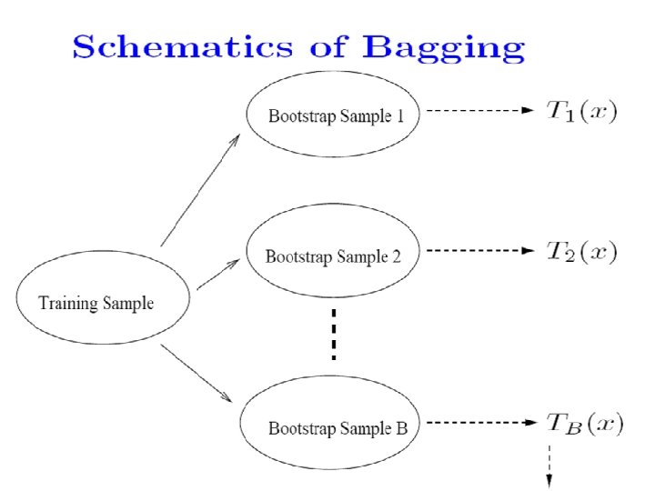
Bootstrap Samples • Sample with replacement. • Training data (y 1, x 1), …. (yn, xn). • Randomly draw one, denote as (y 1*, x 1*); make a copy and put it back. • Repeat for n times, then we have (y 1*, x 1*)…. . (yn*, xn*). This is called a bootstrap sample. • Repeat everything for B times, then we have B bootstrap samples.

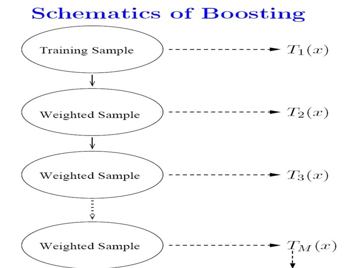
Ensemble Classifiers • Bagging (Breiman 1996): Fit many large trees to bootstrap resampled versions of the training data, and classify by majority vote. • Boosting (Freund & Schapire 1996): Fit many large or small trees to reweighted versions of the training data. Classify by weighted majority vote.

In general, Boosting > Bagging > Single Tree.

Random Forests • General purpose tool for classification and regression. • Impressive accuracy: about as accurate as support vector machines and neural networks • Capable of handling large datasets • Effectively handles missing values • Gives a wealth of scientifically important insights • A set of trees is a forest.

Out-of-bag data • For each tree in the forest, we select a bootstrap sample from the data. • The bootstrap sample is used to grow the tree. • The remaining data are said to be “out-ofbag” (about 1/3 of the cases) • The out-of-bag (oob) data can serve as a test set for the tree grown on the bootstrap sample.

The oob error estimate • Think of a single case in the training set. • It will be out-of-bag in about 1/3 of the trees. • Each time it is out of bag, pass it down the tree and get a predicted class. • The RF prediction is the class that is chosen the most often. • For each case, the RF prediction is either correct or incorrect – Average over the cases within each class to get a classwise oob error rate – Average over all cases to get an overall oob error rate

Out-of-bag data and variable importance • Consider a single tree (fit to a bootstrap sample). 1. Use the tree to predict the class of each out-of-bag case. 2. Randomly permute the values of the variable of interest in all the out-of-bag cases, and use the tree to predict the class for these perturbed out-of-bag cases. The variable importance is the increase in the misclassification rate between steps 1 and 2, averaged over all trees in a forest

Tree and Random Forests Resources • RPART (R interface) • Random. Forest (R interface: Andy Liaw & Matthew Weiner) • Free, open-source code (fortran, java) www. stat. berkeley. edu/users/breiman/R andom. Forests

R implementation • Continuous Y error is RSS • In method=anova, you choose the split that maximizes “between SS” of the two resultant groups • Each group has a prediction equal to the group mean • The error at each node is the variance of y

Variable Importance (in rpart) • Each X can appear multiple times in a tree as primary variables for a split • Also, it can help predict the grouping based on the primary variable if it was missing. “surrogate variable” • VI is a weighted measure of goodness of split for each split where X was a primary variable and for all splits it was a surrogate. (scaled to add up to 100)

library('rpart') ##Grow the tree set. seed(0) #set up the random-number-generator seed for cross validation (CV) fit. cart=rpart(y~. , data=dat. nas, method="anova") # anova for y is continuous, the default CV is 10 -fold. summary(fit. cart) #detailed results fit. cart$cptable# the Complexity parameter (CP)table CP nsplit rel error xstd 1 0. 0362 0 1. 000 1. 00 0. 113 2 0. 0268 3 0. 891 1. 06 0. 113 3 0. 0244 5 0. 838 1. 09 0. 115 4 0. 0216 6 0. 813 1. 10 0. 116 5 0. 0161 8 0. 770 1. 11 0. 119 6 0. 0137 10 0. 738 1. 11 0. 116 7 0. 0120 11 0. 725 1. 12 0. 116 8 0. 0120 12 0. 712 1. 12 0. 116 9 0. 0109 13 0. 701 1. 12 0. 116 10 0. 0107 14 0. 690 1. 14 0. 115 11 0. 0100 15 0. 679 1. 14 0. 115

> plotcp(fit. cart) #plot of CP table

> rpart. plot(fit. cart, type=4, extra = 101, prefix="mean Y=", main="Y=bloodpb") #tree plot Tree corresponding to Complexity parameter=0. 01

vi. cart=fit. cart$variable. importance/sum(fit. cart$variable. importance)*100 #the variable importance, rescaled to add to 100. vi. cart trig serphos calcium chol waistcir k 11. 440 11. 043 10. 497 7. 679 6. 518 4. 368 bmi weight sbp uric hdl hipcir 4. 214 3. 853 3. 244 3. 134 3. 045 2. 729 age sodium educ smokyrs 2. 704 2. 515 2. 495 2. 334 pp calor packyrs calc_wo smk height 2. 307 2. 148 2. 141 2. 083 2. 074 1. 607 hct wcollar hgb dbp htnfam kcaltot 1. 335 1. 078 1. 050 0. 726 0. 519 0. 321 htn white gluc_fas 0. 272 0. 266 0. 261

> length(vi. cart) # number of variables with non-zero variable importance (VI) [1] 31 > sum(vi. cart>1) #number of variables with VI>1 [1] 25 (2) Prune the tree R code: ##Prune the tree prune. cart = prune(fit. cart, cp= fit. cart$cptable[4, "CP"])# prune the tree rpart. plot(prune. cart, type=4, extra = 101, prefix="mean Y=", main="Y=bloodpb") #tree plot vi. prune=prune. cart$variable. importance/sum(prune. cart$variable. importance)*100 #the variable importance, rescaled to add to 100. vi. prune length(vi. prune) # number of variables with non-zero variable importance (VI)

Pruned Tree

> #the variable importance, rescaled to add to 100. > vi. prune serphos chol calcium trig waistcir 18. 577461 13. 578202 12. 832810 11. 030685 10. 370960 weight hipcir bmi hdl age 7. 778220 5. 508537 5. 185480 4. 212198 3. 889110 hct hgb sodium uric height 2. 146413 1. 918071 1. 324382 0. 323088 > length(vi. prune) # number of variables with non-zero variable importance (VI) [1] 15 Remark: There are only 15 variables with non-zero variable importance after pruning the tree.

Ensemble Learning •

How to choose/estimate the optimal weights? • Again resort to cross-validation • Asymptotically optimal with a convex combination of predictions and a bounded loss function (Polley and vam der Laan, 2011) • Similar to the idea of stacking used in Neural Networks

Library of learners