Classification and Prediction Data Mining Concepts and Techniques

Classification and Prediction (Data Mining: Concepts and Techniques) 2021/2/27 Data Mining: Concepts and Techniques 1

Chapter 6 Classification and Prediction n n n n 2021/2/27 What is classification? What is prediction? Issues regarding classification and prediction Classification by decision tree induction Bayesian Classification by backpropagation Other Classification Methods Prediction Performance evaluation Summary Data Mining: Concepts and Techniques 2

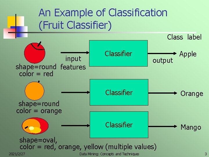
An Example of Classification (Fruit Classifier) Class label input shape=round features color = red Classifier output Apple Classifier Orange Classifier Mango shape=round color = orange shape=oval, color = red, orange, yellow (multiple values) 2021/2/27 Data Mining: Concepts and Techniques 3

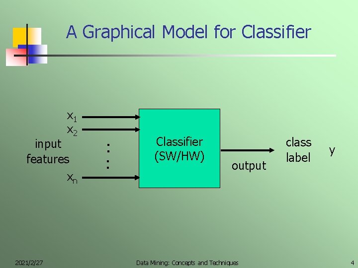
A Graphical Model for Classifier x 1 x 2 input features xn 2021/2/27 : : Classifier (SW/HW) output Data Mining: Concepts and Techniques class label y 4

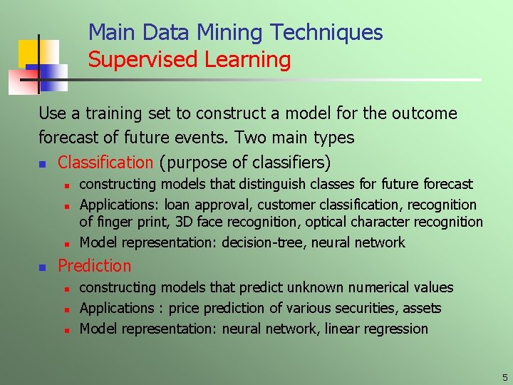
Main Data Mining Techniques Supervised Learning Use a training set to construct a model for the outcome forecast of future events. Two main types n Classification (purpose of classifiers) n n constructing models that distinguish classes for future forecast Applications: loan approval, customer classification, recognition of finger print, 3 D face recognition, optical character recognition Model representation: decision-tree, neural network Prediction n constructing models that predict unknown numerical values Applications : price prediction of various securities, assets Model representation: neural network, linear regression 5

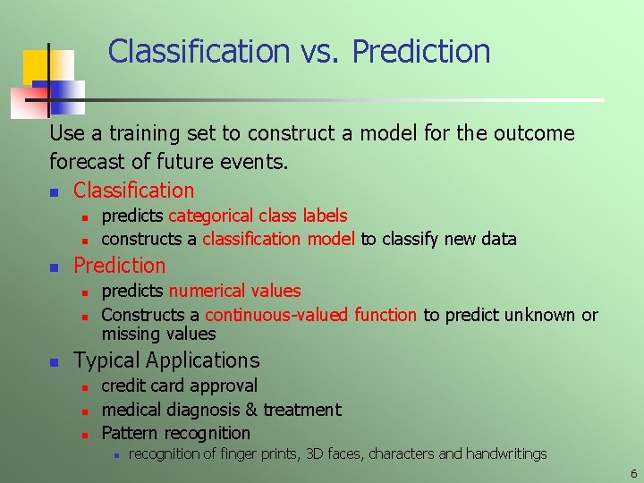
Classification vs. Prediction Use a training set to construct a model for the outcome forecast of future events. n Classification n Prediction n predicts categorical class labels constructs a classification model to classify new data predicts numerical values Constructs a continuous-valued function to predict unknown or missing values Typical Applications n n n credit card approval medical diagnosis & treatment Pattern recognition of finger prints, 3 D faces, characters and handwritings 6

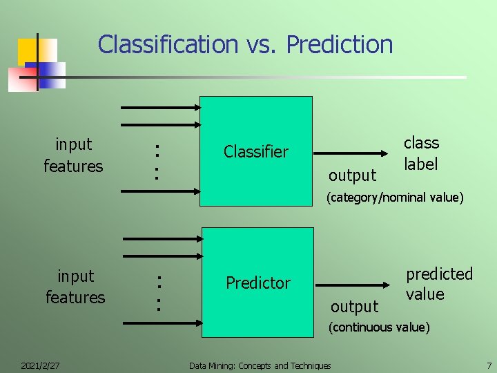
Classification vs. Prediction input features : : Classifier output class label (category/nominal value) input features : : Predictor output predicted value (continuous value) 2021/2/27 Data Mining: Concepts and Techniques 7

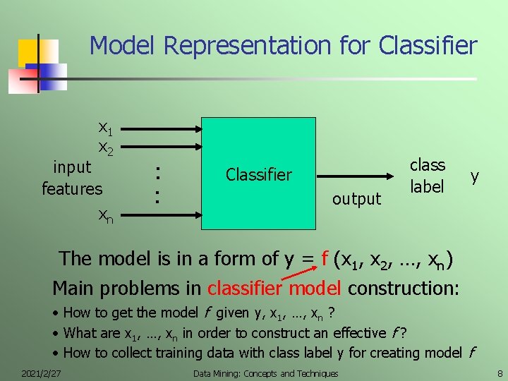
Model Representation for Classifier x 1 x 2 input features xn : : Classifier output class label y The model is in a form of y = f (x 1, x 2, …, xn) Main problems in classifier model construction: • How to get the model f given y, x 1, …, xn ? • What are x 1, …, xn in order to construct an effective f ? • How to collect training data with class label y for creating model f 2021/2/27 Data Mining: Concepts and Techniques 8

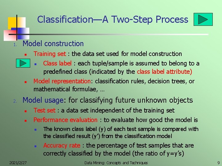
Classification—A Two-Step Process 1. Model construction n Training set : the data set used for model construction n n 2. Class label : each tuple/sample is assumed to belong to a predefined class (indicated by the class label attribute) Model representation: classification rules, decision trees, or mathematical formulae, … Model usage: for classifying future unknown objects n Test set : a data set independent of the training set n Performance evaluation : to evaluate how good the model is n n 2021/2/27 The known class label (y) of each test sample is compared with the classified result (y’) from the classification model Accuracy rate : the percentage of test samples that are correctly classified by the model (the ratio of y=y’s) Data Mining: Concepts and Techniques 9

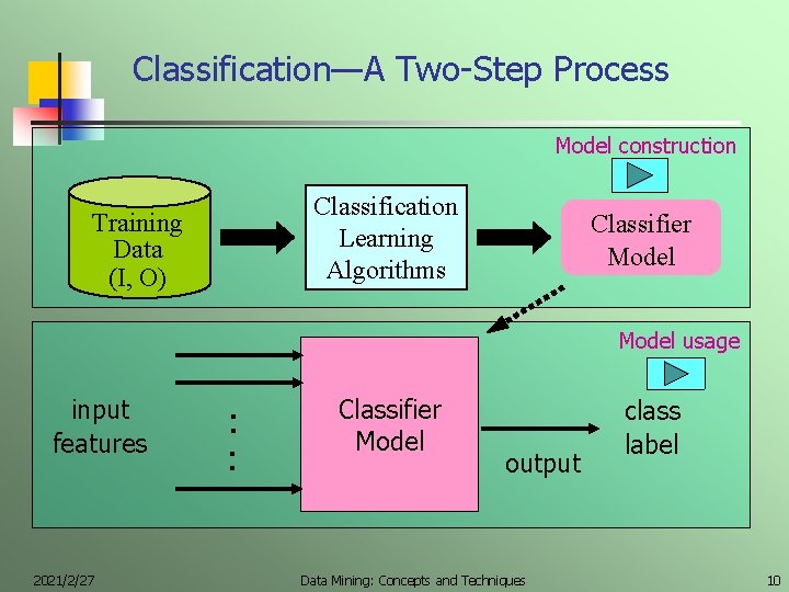
Classification—A Two-Step Process Model construction Classification Learning Algorithms Training Data (I, O) Classifier Model usage input features 2021/2/27 : : Classifier Model output Data Mining: Concepts and Techniques class label 10

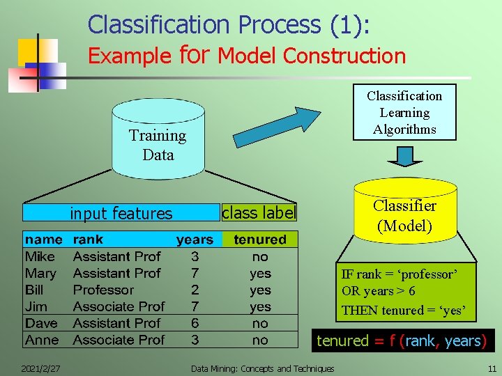
Classification Process (1): Example for Model Construction Classification Learning Algorithms Training Data input features Classifier (Model) class label IF rank = ‘professor’ OR years > 6 THEN tenured = ‘yes’ tenured = f (rank, years) 2021/2/27 Data Mining: Concepts and Techniques 11

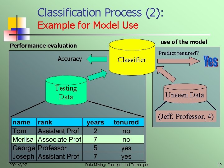
Classification Process (2): Example for Model Use use of the model Performance evaluation Accuracy Classifier Testing Data Predict tenured? Unseen Data (Jeff, Professor, 4) 2021/2/27 Data Mining: Concepts and Techniques 12

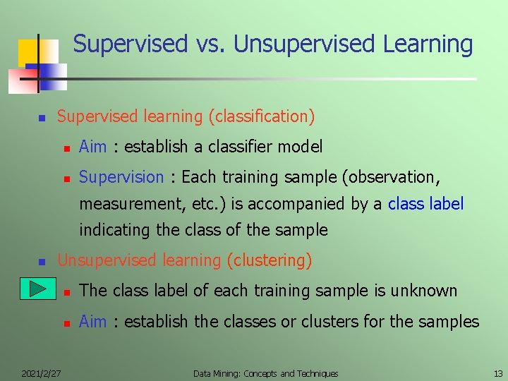
Supervised vs. Unsupervised Learning n Supervised learning (classification) n Aim : establish a classifier model n Supervision : Each training sample (observation, measurement, etc. ) is accompanied by a class label indicating the class of the sample n Unsupervised learning (clustering) 2021/2/27 n The class label of each training sample is unknown n Aim : establish the classes or clusters for the samples Data Mining: Concepts and Techniques 13

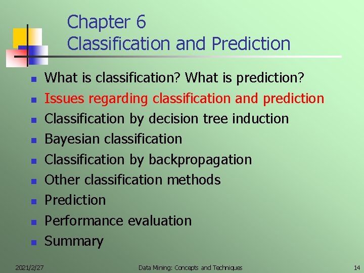
Chapter 6 Classification and Prediction n n n n 2021/2/27 What is classification? What is prediction? Issues regarding classification and prediction Classification by decision tree induction Bayesian classification Classification by backpropagation Other classification methods Prediction Performance evaluation Summary Data Mining: Concepts and Techniques 14

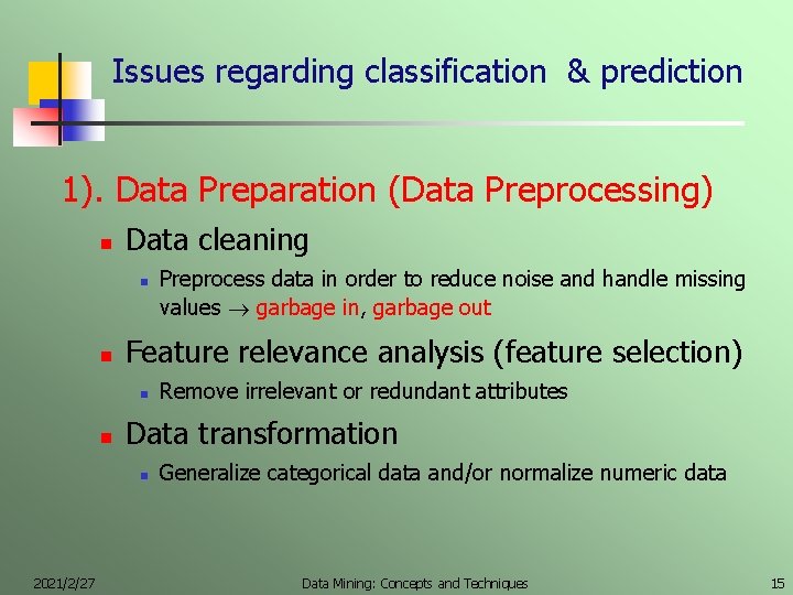
Issues regarding classification & prediction 1). Data Preparation (Data Preprocessing) n Data cleaning n n Feature relevance analysis (feature selection) n n Remove irrelevant or redundant attributes Data transformation n 2021/2/27 Preprocess data in order to reduce noise and handle missing values garbage in, garbage out Generalize categorical data and/or normalize numeric data Data Mining: Concepts and Techniques 15

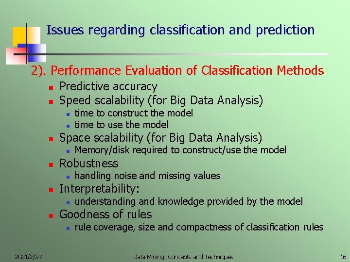
Issues regarding classification and prediction 2). Performance Evaluation of Classification Methods n n Predictive accuracy Speed scalability (for Big Data Analysis) n n n Space scalability (for Big Data Analysis) n n understanding and knowledge provided by the model Goodness of rules n 2021/2/27 handling noise and missing values Interpretability: n n Memory/disk required to construct/use the model Robustness n n time to construct the model time to use the model rule coverage, size and compactness of classification rules Data Mining: Concepts and Techniques 16

Chapter 6 Classification and Prediction n n n n 2021/2/27 What is classification? What is prediction? Issues regarding classification and prediction Classification by decision tree induction Bayesian classification Classification by backpropagation Other classification methods Prediction Performance evaluation Summary Data Mining: Concepts and Techniques 17

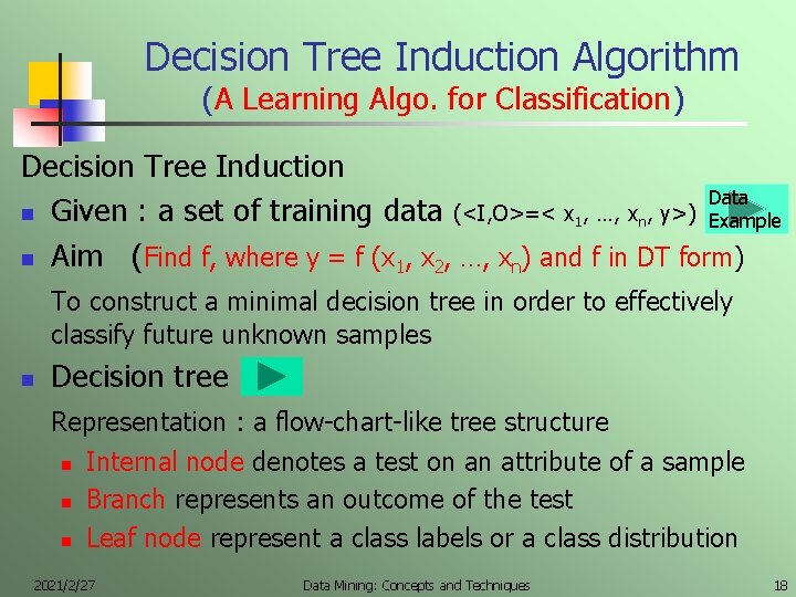
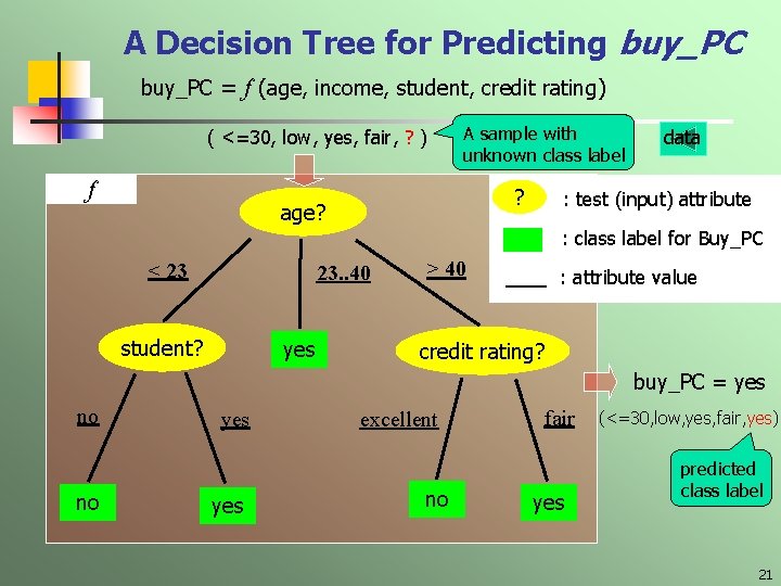
Decision Tree Induction Algorithm (A Learning Algo. for Classification) Decision Tree Induction Data n Given : a set of training data (<I, O>=< x 1, …, xn, y>) Example n Aim (Find f, where y = f (x 1, x 2, …, xn) and f in DT form) To construct a minimal decision tree in order to effectively classify future unknown samples n Decision tree Representation : a flow-chart-like tree structure n Internal node denotes a test on an attribute of a sample n Branch represents an outcome of the test n Leaf node represent a class labels or a class distribution 2021/2/27 Data Mining: Concepts and Techniques 18

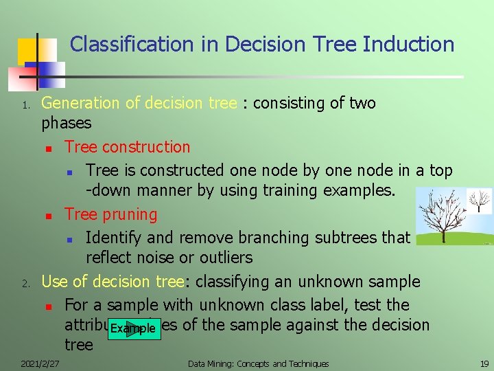
Classification in Decision Tree Induction 1. 2. Generation of decision tree : consisting of two phases n Tree construction n Tree is constructed one node by one node in a top -down manner by using training examples. n Tree pruning n Identify and remove branching subtrees that reflect noise or outliers Use of decision tree: classifying an unknown sample n For a sample with unknown class label, test the attribute values of the sample against the decision Example tree 2021/2/27 Data Mining: Concepts and Techniques 19

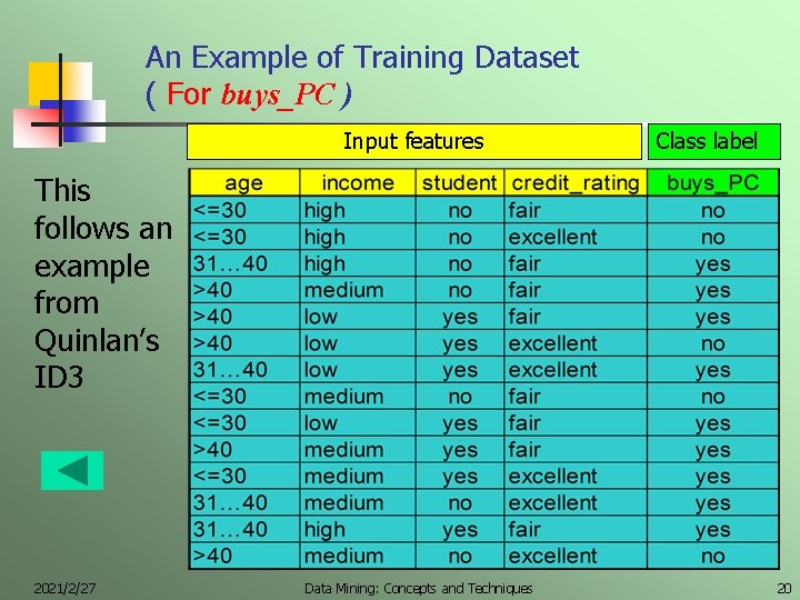
An Example of Training Dataset ( For buys_PC ) Input features Class label This follows an example from Quinlan’s ID 3 2021/2/27 Data Mining: Concepts and Techniques 20

A Decision Tree for Predicting buy_PC = f (age, income, student, credit rating) ( <=30, low, yes, fair, ? ) f A sample with unknown class label ? age? data : test (input) attribute : class label for Buy_PC < 23 23. . 40 student? yes > 40 : attribute value credit rating? buy_PC = yes no no yes excellent no fair yes (<=30, low, yes, fair, yes) predicted class label 21

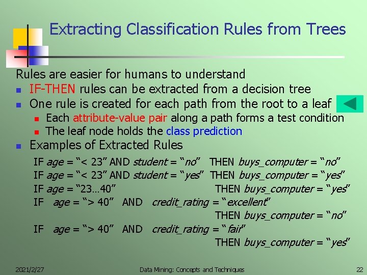
Extracting Classification Rules from Trees Rules are easier for humans to understand n IF-THEN rules can be extracted from a decision tree n One rule is created for each path from the root to a leaf n n n Each attribute-value pair along a path forms a test condition The leaf node holds the class prediction Examples of Extracted Rules age = “< 23” AND student = “no” THEN buys_computer = “no” age = “< 23” AND student = “yes” THEN buys_computer = “yes” age = “ 23… 40” THEN buys_computer = “yes” age = “> 40” AND credit_rating = “excellent” THEN buys_computer = “no” IF age = “> 40” AND credit_rating = “fair” THEN buys_computer = “yes” IF IF 2021/2/27 Data Mining: Concepts and Techniques 22

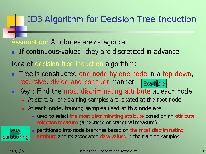
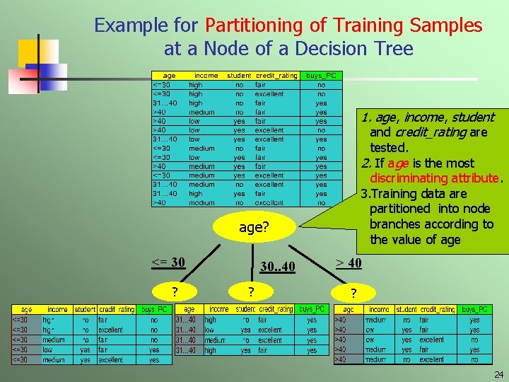
ID 3 Algorithm for Decision Tree Induction Assumption: Attributes are categorical n If continuous-valued, they are discretized in advance Idea of decision tree induction algorithm: n Tree is constructed one node by one node in a top-down, recursive, divide-and-conquer manner Example n Key : Find the most discriminating attribute at each node n n At start, all the training samples are located at the root node At each node, training samples used at this node are n Data partitioning 2021/2/27 n used to select the most discriminating attribute based on an attribute selection measure (a heuristic or statistical measure) partitioned into node branches based on the most discriminating attribute and its associated data values in the training samples Data Mining: Concepts and Techniques 23

Example for Partitioning of Training Samples at a Node of a Decision Tree 1. age, income, student and credit_rating are tested. 2. If age is the most discriminating attribute. 3. Training data are partitioned into node branches according to the value of age? <= 30 ? 30. . 40 ? > 40 ? 24

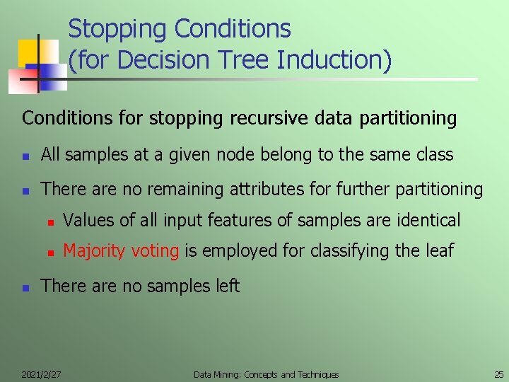
Stopping Conditions (for Decision Tree Induction) Conditions for stopping recursive data partitioning n All samples at a given node belong to the same class n There are no remaining attributes for further partitioning n n Values of all input features of samples are identical n Majority voting is employed for classifying the leaf There are no samples left 2021/2/27 Data Mining: Concepts and Techniques 25

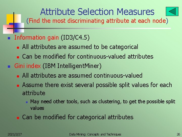
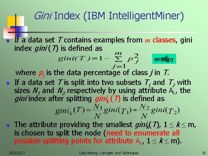
Attribute Selection Measures (Find the most discriminating attribute at each node) n n Information gain (ID 3/C 4. 5) n All attributes are assumed to be categorical n Can be modified for continuous-valued attributes Gini index (IBM Intelligent. Miner) n n All attributes are assumed continuous-valued Assume there exist several possible split values for each attribute n n 2021/2/27 May need other tools, such as clustering, to get the possible split values Can be modified for categorical attributes Data Mining: Concepts and Techniques 26

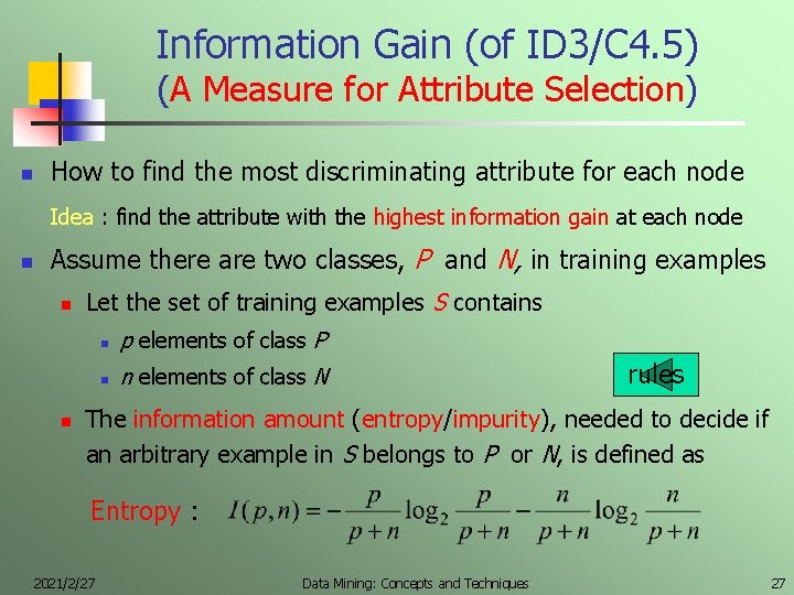
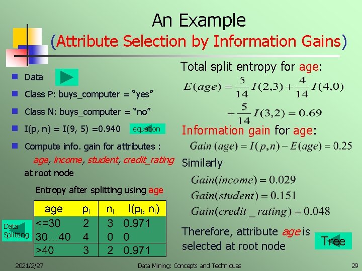
Information Gain (of ID 3/C 4. 5) (A Measure for Attribute Selection) n How to find the most discriminating attribute for each node Idea : find the attribute with the highest information gain at each node n Assume there are two classes, P and N, in training examples n n Let the set of training examples S contains n p elements of class P n n elements of class N rules The information amount (entropy/impurity), needed to decide if an arbitrary example in S belongs to P or N, is defined as Entropy : 2021/2/27 Data Mining: Concepts and Techniques 27

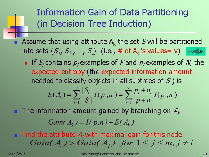
Information Gain of Data Partitioning (in Decision Tree Induction) n Assume that using attribute Ak the set S will be partitioned into sets {S 1, S 2 , …, Sv} (i. e. , # of Ak ’s values= v) Example n If Si contains pi examples of P and ni examples of N, the expected entropy (the expected information amount needed to classify objects in all subtrees of S ) is n The information amount gained by branching on Ak n Find the attribute Ai with maximal gain for this node 2021/2/27 Data Mining: Concepts and Techniques 28

An Example (Attribute Selection by Information Gains) Total split entropy for age: g Data g Class P: buys_computer = “yes” g Class N: buys_computer = “no” g I(p, n) = I(9, 5) =0. 940 g Compute info. gain for attributes : equation Information gain for age: age, income, student, credit_rating Similarly at root node Entropy after splitting using age Data Splitting 2021/2/27 Therefore, attribute age is selected at root node Data Mining: Concepts and Techniques Tree 29

Gini Index (IBM Intelligent. Miner) n If a data set T contains examples from m classes, gini index gini (T) is defined as entropy n n where pj is the data percentage of class j in T. If a data set T is split into two subsets T 1 and T 2 with sizes N 1 and N 2 respectively by using attribute Ak, the gini index after splitting ginik (T) is defined as The attribute providing the smallest ginik(T), 1 ≤ k ≤ m, is chosen to split the node (need to enumerate all possible splitting points for attribute Ak, 1 ≤ k ≤ m). 2021/2/27 Data Mining: Concepts and Techniques 30

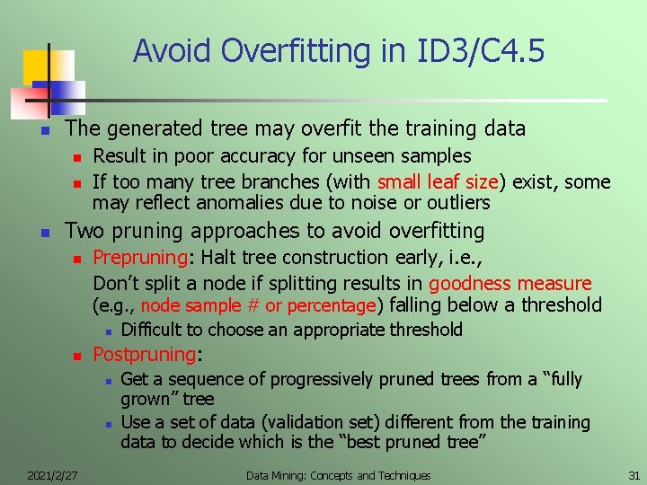
Avoid Overfitting in ID 3/C 4. 5 n The generated tree may overfit the training data n n n Result in poor accuracy for unseen samples If too many tree branches (with small leaf size) exist, some may reflect anomalies due to noise or outliers Two pruning approaches to avoid overfitting n Prepruning: Halt tree construction early, i. e. , Don’t split a node if splitting results in goodness measure (e. g. , node sample # or percentage) falling below a threshold n n Postpruning: n n 2021/2/27 Difficult to choose an appropriate threshold Get a sequence of progressively pruned trees from a “fully grown” tree Use a set of data (validation set) different from the training data to decide which is the “best pruned tree” Data Mining: Concepts and Techniques 31

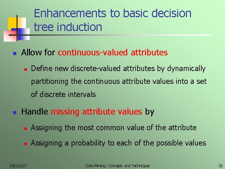
Enhancements to basic decision tree induction n Allow for continuous-valued attributes n Define new discrete-valued attributes by dynamically partitioning the continuous attribute values into a set of discrete intervals n Handle missing attribute values by n Assigning the most common value of the attribute n Assigning a probability to each of the possible values 2021/2/27 Data Mining: Concepts and Techniques 32

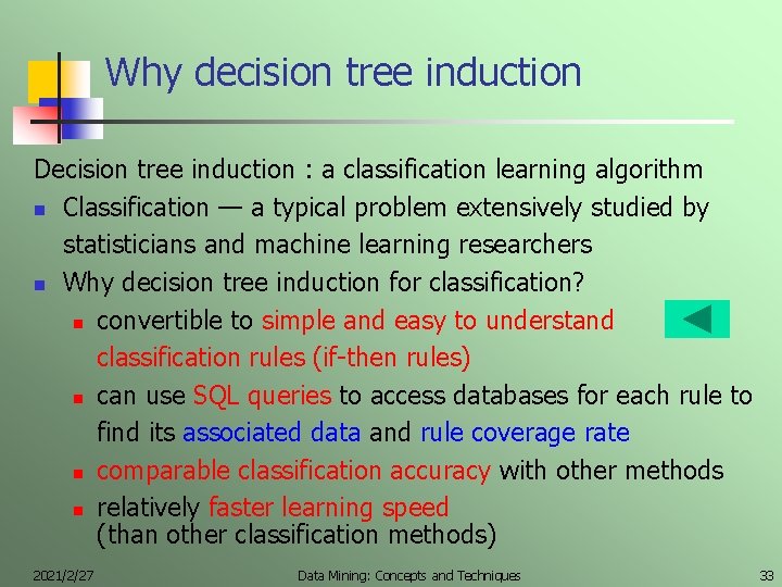
Why decision tree induction Decision tree induction : a classification learning algorithm n Classification — a typical problem extensively studied by statisticians and machine learning researchers n Why decision tree induction for classification? n convertible to simple and easy to understand classification rules (if-then rules) n can use SQL queries to access databases for each rule to find its associated data and rule coverage rate n comparable classification accuracy with other methods n relatively faster learning speed (than other classification methods) 2021/2/27 Data Mining: Concepts and Techniques 33

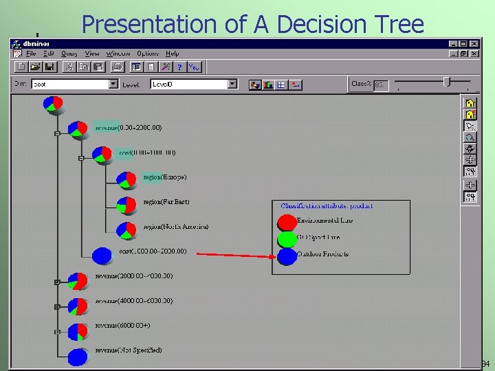
Presentation of A Decision Tree 2021/2/27 Data Mining: Concepts and Techniques 34

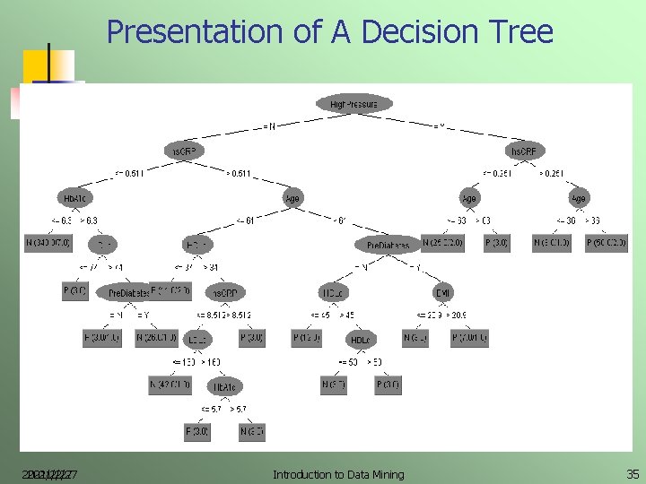
Presentation of A Decision Tree 2021/2/27 Introduction to Data Mining 35

Chapter 6 Classification and Prediction n n 2021/2/27 What is classification? What is prediction? Issues regarding classification and prediction Classification by decision tree induction Bayesian Classification by backpropagation Classification based on concepts from association rule mining Other Classification Methods Prediction Performance evaluation Summary Data Mining: Concepts and Techniques 36

Bayesian Classification: Why? n n Probabilistic prediction and learning: n Predict multiple hypotheses n Calculate a probability for each hypothesis Incremental learning : n n n Each training example incrementally increases/decreases the probability that a hypothesis is correct. Prior knowledge can be combined with observed data. Benchmark standard: Even when Bayesian methods are computationally intractable, they can provide a benchmark standard against other methods 2021/2/27 Data Mining: Concepts and Techniques 37

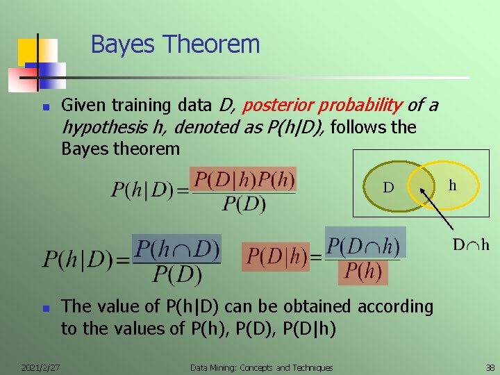
Bayes Theorem n Given training data D, posterior probability of a hypothesis h, denoted as P(h|D), follows the Bayes theorem D n 2021/2/27 h The value of P(h|D) can be obtained according to the values of P(h), P(D|h) Data Mining: Concepts and Techniques 38

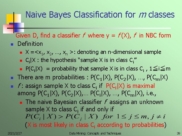
Naive Bayes Classification for m classes n Given D, find a classifier f where y = f (X), f in NBC form Definition n X =<x 1, x 2, …, xn >: denoting an n-dimensional sample Ci|X : the hypothesis “sample X is in class Ci” n P(Ci|X) = probability that sample X is in class Ci , 1≦i≦m n n n There are m probabilities : P(C 1|X), P(C 2|X), …, P(Cm|X) f : assign sample X to class Ci if P(Ci|X) is maximal among P(C 1|X), P(C 2|X), … P(Ci|X), …, P(Cm|X), i. e. , n The naive Bayesian classifier f assigns an unknown sample X to class Ci if and only if (X is most likely in class Ci according to probabilities) 2021/2/27 Data Mining: Concepts and Techniques 39

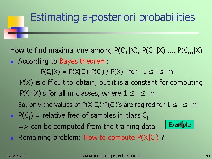
Estimating a-posteriori probabilities How to find maximal one among P(C 1|X), P(C 2|X) …, P(Cm|X) n According to Bayes theorem: P(Ci|X) = P(X|Ci)·P(Ci) / P(X) for 1 ≤ i ≤ m P(X) is difficult to obtain, but it is a constant for computing P(Ci|X)’s for all m classes, where 1 ≤ i ≤ m So, only the values of P(X|Ci)·P(Ci)’s are reqired for 1 ≤ i ≤ m n P(Ci) = relative freq of samples in class Ci => can be computed from the training data n Example Remaining problem: How to compute P(X|Ci) ? 2021/2/27 Data Mining: Concepts and Techniques 40

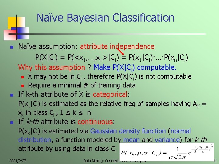
Naïve Bayesian Classification n Naïve assumption: attribute independence P(X|Ci) = P(<x 1, …, xn>|Ci) = P(x 1|Ci)·…·P(xn|Ci) Why this assumption ? Make P(X|Ci) computable. n n n X may not be in Ci , therefore P(X|Ci) is not computable Require a minimal # of training data If k-th attribute of X is categorical: P(xk|Ci) is estimated as the relative freq of samples having Ak’ = xk in class Ci , 1 ≤ k ≤ n n If k-th attribute is continuous: P(xk|Ci) is estimated via Gaussian density function (normal distribution, a function modeled by mean and variance) for k-th attribute by using data in class Ci 2021/2/27 Data Mining: Concepts and Techniques 41

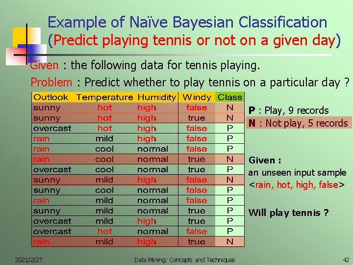
Example of Naïve Bayesian Classification (Predict playing tennis or not on a given day) Given : the following data for tennis playing. Problem : Predict whether to play tennis on a particular day ? P : Play, 9 records N : Not play, 5 records Given : an unseen input sample <rain, hot, high, false> Will play tennis ? 2021/2/27 Data Mining: Concepts and Techniques 42

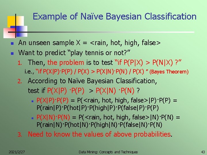
Example of Naïve Bayesian Classification n n An unseen sample X = <rain, hot, high, false> Want to predict “play tennis or not? ” 1. Then, the problem is to test “if P(P|X) > P(N|X) ? ” i. e. , “if P(X|P)·P(P) / P(X) > P(X|N)·P(N) / P(X) ” (Bayes Theorem) 2. According to Naïve Bayesian Classification, test if P(X|P) ·P(P) > P(X|N) ·P(N) ? n n 3. 2021/2/27 P(X|P)·P(P) = P(<rain, hot, high, false>|P)·P(P) = P(rain|P)·P(hot|P)·P(high|P)·P(false|P)·P(P) P(X|N)·P(N) = P(<rain, hot, high, false>|N)·P(N) = P(rain|N)·P(hot|N)·P(high|N)·P(false|N)·P(N) Need to know the values of above probabilities. Data Mining: Concepts and Techniques 43

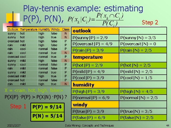
Play-tennis example: estimating P(P), P(N), Step 2 outlook P(sunny|P) = 2/9 P(sunny|N) = 3/5 P(overcast|P) = 4/9 P(overcast|N) = 0 P(rain|P) = 3/9 P(rain|N) = 2/5 temperature X = <rain, hot, high, false> P(X|P) ·P(P) > P(X|N) ·P(N) ? Step 1 P(P) = 9/14 P(N) = 5/14 2021/2/27 P(hot|P) = 2/9 P(hot|N) = 2/5 P(mild|P) = 4/9 P(mild|N) = 2/5 P(cool|P) = 3/9 P(cool|N) = 1/5 humidity P(high|P) = 3/9 P(high|N) = 4/5 P(normal|P) = 6/9 P(normal|N) = 2/5 windy P(true|P) = 3/9 P(true|N) = 3/5 P(false|P) = 6/9 P(false|N) = 2/5 Data Mining: Concepts and Techniques 44

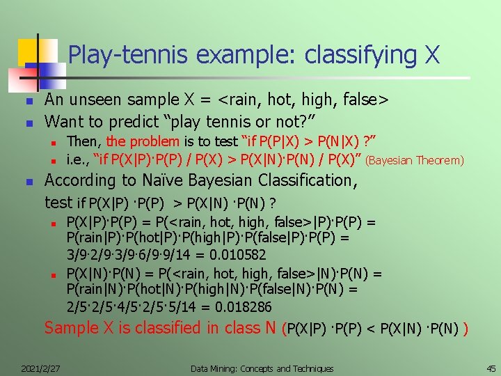
Play-tennis example: classifying X n n An unseen sample X = <rain, hot, high, false> Want to predict “play tennis or not? ” n n n Then, the problem is to test “if P(P|X) > P(N|X) ? ” i. e. , “if P(X|P)·P(P) / P(X) > P(X|N)·P(N) / P(X)” (Bayesian Theorem) According to Naïve Bayesian Classification, test if P(X|P) ·P(P) > P(X|N) ·P(N) ? n n P(X|P)·P(P) = P(<rain, hot, high, false>|P)·P(P) = P(rain|P)·P(hot|P)·P(high|P)·P(false|P)·P(P) = 3/9· 2/9· 3/9· 6/9· 9/14 = 0. 010582 P(X|N)·P(N) = P(<rain, hot, high, false>|N)·P(N) = P(rain|N)·P(hot|N)·P(high|N)·P(false|N)·P(N) = 2/5· 4/5· 2/5· 5/14 = 0. 018286 Sample X is classified in class N (P(X|P) ·P(P) < P(X|N) ·P(N) ) 2021/2/27 Data Mining: Concepts and Techniques 45

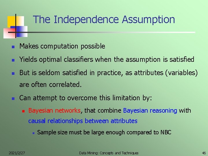
The Independence Assumption n Makes computation possible n Yields optimal classifiers when the assumption is satisfied n But is seldom satisfied in practice, as attributes (variables) are often correlated. n Can attempt to overcome this limitation by: n Bayesian networks, that combine Bayesian reasoning with causal relationships between attributes n 2021/2/27 Sample size must be large enough compared to NBC Data Mining: Concepts and Techniques 46

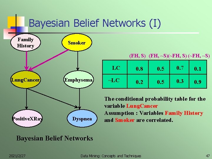
Bayesian Belief Networks (I) Family History Smoker (FH, S) (FH, ~S)(~FH, S) (~FH, ~S) Lung. Cancer Positive. XRay Emphysema Dyspnea LC 0. 8 0. 5 0. 7 0. 1 ~LC 0. 2 0. 5 0. 3 0. 9 The conditional probability table for the variable Lung. Cancer Assumption : Variables Family History and Smoker are correlated. Bayesian Belief Networks 2021/2/27 Data Mining: Concepts and Techniques 47

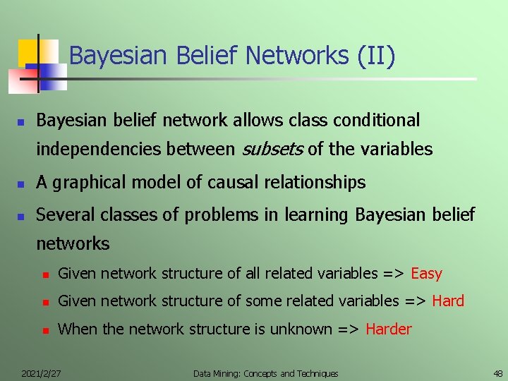
Bayesian Belief Networks (II) n Bayesian belief network allows class conditional independencies between subsets of the variables n A graphical model of causal relationships n Several classes of problems in learning Bayesian belief networks n Given network structure of all related variables => Easy n Given network structure of some related variables => Hard n When the network structure is unknown => Harder 2021/2/27 Data Mining: Concepts and Techniques 48

Chapter 6 Classification and Prediction n n n n 2021/2/27 What is classification? What is prediction? Issues regarding classification and prediction Classification by decision tree induction Bayesian classification Discriminative classification Other classification methods Prediction Performance evaluation Summary Data Mining: Concepts and Techniques 49

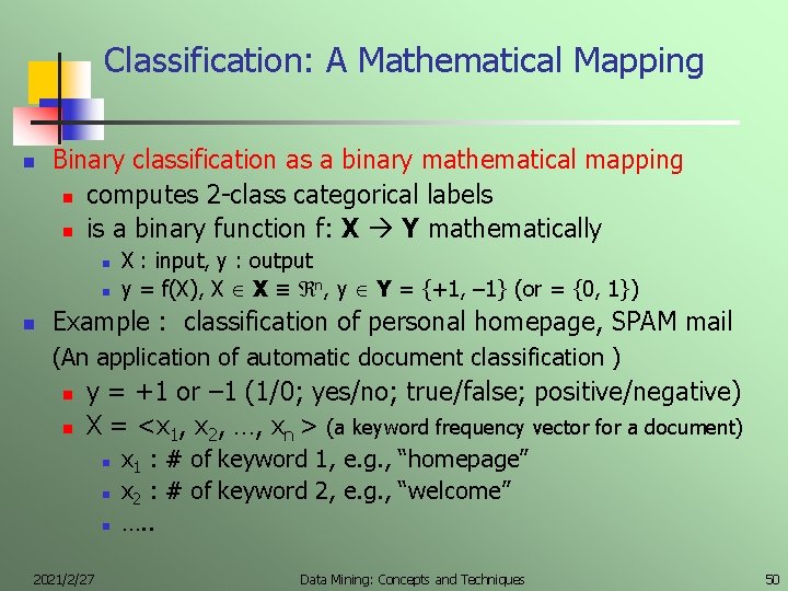
Classification: A Mathematical Mapping n Binary classification as a binary mathematical mapping n computes 2 -class categorical labels n is a binary function f: X Y mathematically n n n X : input, y : output y = f(X), X X ≡ n, y Y = {+1, – 1} (or = {0, 1}) Example : classification of personal homepage, SPAM mail (An application of automatic document classification ) n n y = +1 or – 1 (1/0; yes/no; true/false; positive/negative) X = <x 1, x 2, …, xn > (a keyword frequency vector for a document) n n n 2021/2/27 x 1 : # of keyword 1, e. g. , “homepage” x 2 : # of keyword 2, e. g. , “welcome” …. . Data Mining: Concepts and Techniques 50

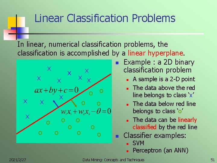
Linear Classification Problems In linear, numerical classification problems, the classification is accomplished by a linear hyperplane. n Example : a 2 D binary x classification problem x x x n A sample is a 2 -D point x n The data above the red o o line belongs to class ‘x’ x x x o o n The data below red line x o o o o n o n Classifier examples: n n 2021/2/27 belongs to class ‘o’ The data can be linearly classified by the red line SVM Perceptron (an ANN) Data Mining: Concepts and Techniques 51

Chapter 6 Classification and Prediction n n n n 2021/2/27 What is classification? What is prediction? Issues regarding classification and prediction Classification by decision tree induction Bayesian classification Classification by backpropagation Other classification methods Prediction Estimating classification Summary Data Mining: Concepts and Techniques 52

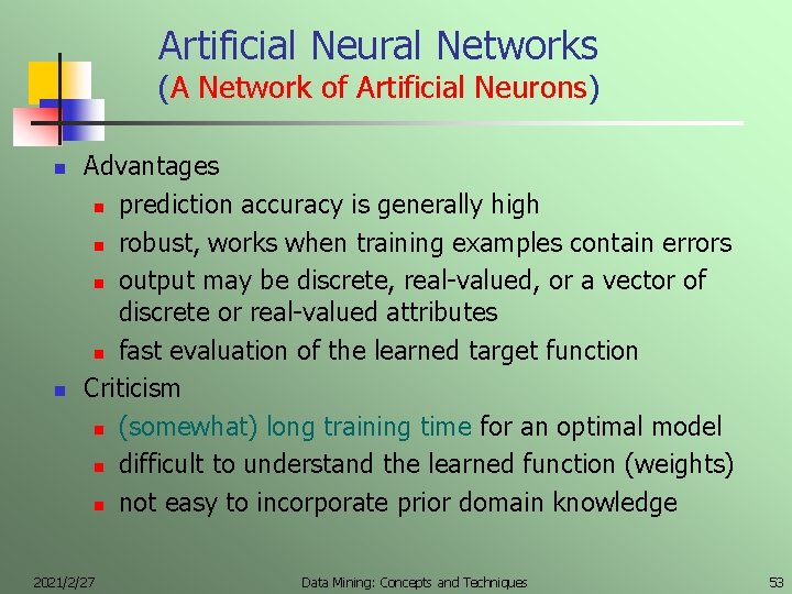
Artificial Neural Networks (A Network of Artificial Neurons) n n Advantages n prediction accuracy is generally high n robust, works when training examples contain errors n output may be discrete, real-valued, or a vector of discrete or real-valued attributes n fast evaluation of the learned target function Criticism n (somewhat) long training time for an optimal model n difficult to understand the learned function (weights) n not easy to incorporate prior domain knowledge 2021/2/27 Data Mining: Concepts and Techniques 53

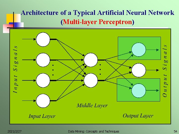
Architecture of a Typical Artificial Neural Network (Multi-layer Perceptron) . . . 2021/2/27 . . . Data Mining: Concepts and Techniques 54

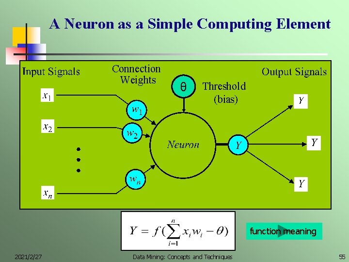
A Neuron as a Simple Computing Element Connection Weights θ Threshold (bias) function meaning 2021/2/27 Data Mining: Concepts and Techniques 55

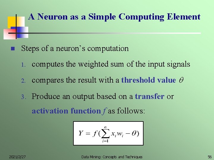
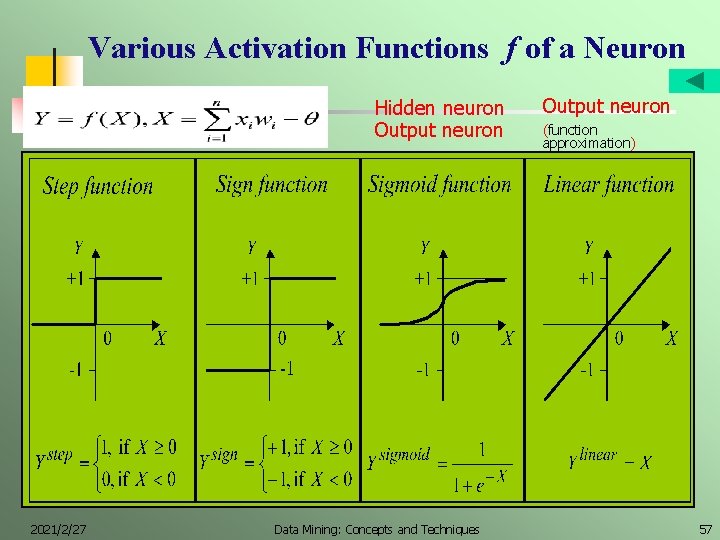
A Neuron as a Simple Computing Element n Steps of a neuron’s computation 1. computes the weighted sum of the input signals 2. compares the result with a threshold value 3. Produce an output based on a transfer or activation function f as follows: 2021/2/27 Data Mining: Concepts and Techniques 56

Various Activation Functions f of a Neuron Hidden neuron Output neuron 2021/2/27 Data Mining: Concepts and Techniques Output neuron (function approximation) 57

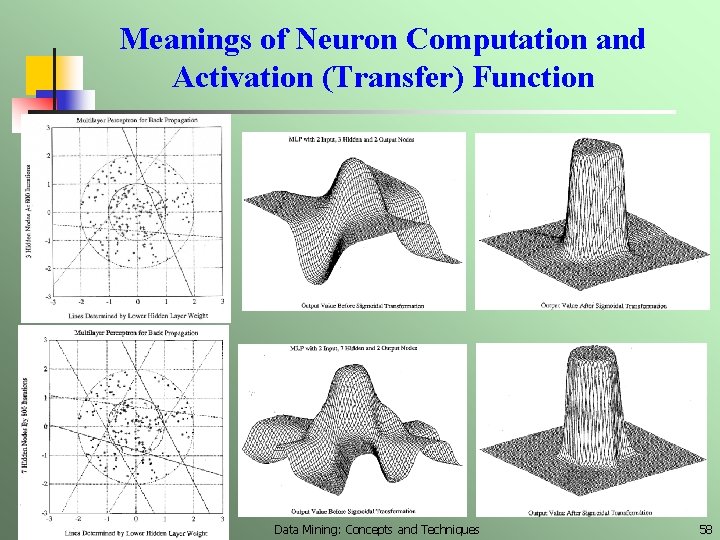
Meanings of Neuron Computation and Activation (Transfer) Function 2021/2/27 Data Mining: Concepts and Techniques 58

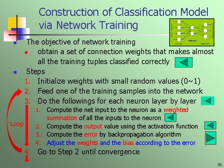
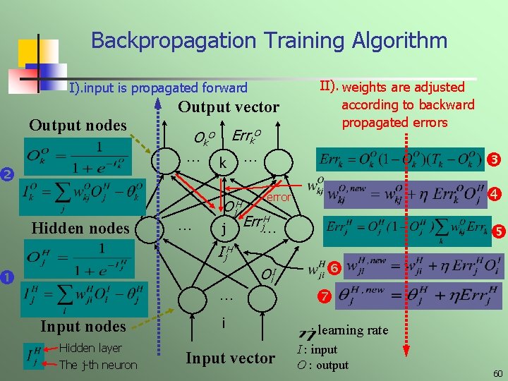
Construction of Classification Model via Network Training n n The objective of network training n obtain a set of connection weights that makes almost all the training tuples classified correctly Steps 1. Initialize weights with small random values (0~1) 2. Feed one of the training samples into the network 3. Do the followings for each neuron layer by layer 1. Loop 2. 3. 4. Compute the net input to the neuron as a weighted summation of all the inputs to the neuron Compute the output value using the activation function Compute the error by backpropagation algorithm Adjust the weights and the bias according to the error Go to Step 2 until convergence 59

Backpropagation Training Algorithm I). input is propagated forward Output nodes Output vector … Hidden nodes Errk. O Ok O … k Oj H j … … Input nodes Hidden layer The j-th neuron error H Errj… Ij H II). weights are adjusted according to backward propagated errors Oi. I i Input vector : learning rate I : input O : output 60

Chapter 6 Classification and Prediction n n n n 2021/2/27 What is classification? What is prediction? Issues regarding classification and prediction Classification by decision tree induction Bayesian classification Classification by backpropagation Other classification methods Prediction Performance evaluation Summary Data Mining: Concepts and Techniques 61

Other Classification Methods n SVM—Support Vector Machines n k-nearest neighbor classifier n Case-based reasoning n Rough set approach n Fuzzy set approaches 2021/2/27 Data Mining: Concepts and Techniques 62

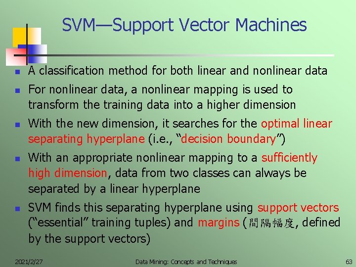
SVM—Support Vector Machines n n n A classification method for both linear and nonlinear data For nonlinear data, a nonlinear mapping is used to transform the training data into a higher dimension With the new dimension, it searches for the optimal linear separating hyperplane (i. e. , “decision boundary”) With an appropriate nonlinear mapping to a sufficiently high dimension, data from two classes can always be separated by a linear hyperplane SVM finds this separating hyperplane using support vectors (“essential” training tuples) and margins (間隔幅度, defined by the support vectors) 2021/2/27 Data Mining: Concepts and Techniques 63

SVM—History and Applications n Vapnik and colleagues (1992)—groundwork from Vapnik & Chervonenkis’ statistical learning theory in 1960 s n Features: training can be slow but accuracy is high owing to their ability to model complex nonlinear decision boundaries (for margin maximization) n Used both for classification and prediction n Applications: n 2021/2/27 handwritten digit recognition, object recognition, speaker identification Data Mining: Concepts and Techniques 64

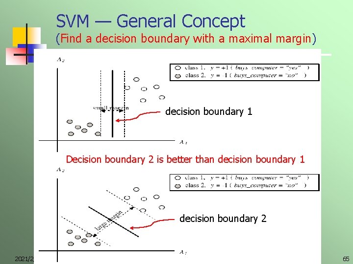
SVM — General Concept (Find a decision boundary with a maximal margin) decision boundary 1 Decision boundary 2 is better than decision boundary 1 decision boundary 2 2021/2/27 Data Mining: Concepts and Techniques 65

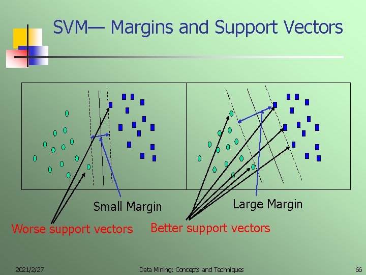
SVM— Margins and Support Vectors Small Margin Worse support vectors 2021/2/27 Large Margin Better support vectors Data Mining: Concepts and Techniques 66

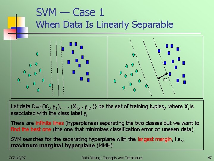
SVM — Case 1 When Data Is Linearly Separable m Let data D={(X 1, y 1), …, (X|D|, y|D|)} be the set of training tuples, where Xi is associated with the class label yi There are infinite lines (hyperplanes) separating the two classes but we want to find the best one (the one that minimizes classification error on unseen data) SVM searches for the separating hyperplane with the largest margin, i. e. , maximum marginal hyperplane (MMH) 2021/2/27 Data Mining: Concepts and Techniques 67

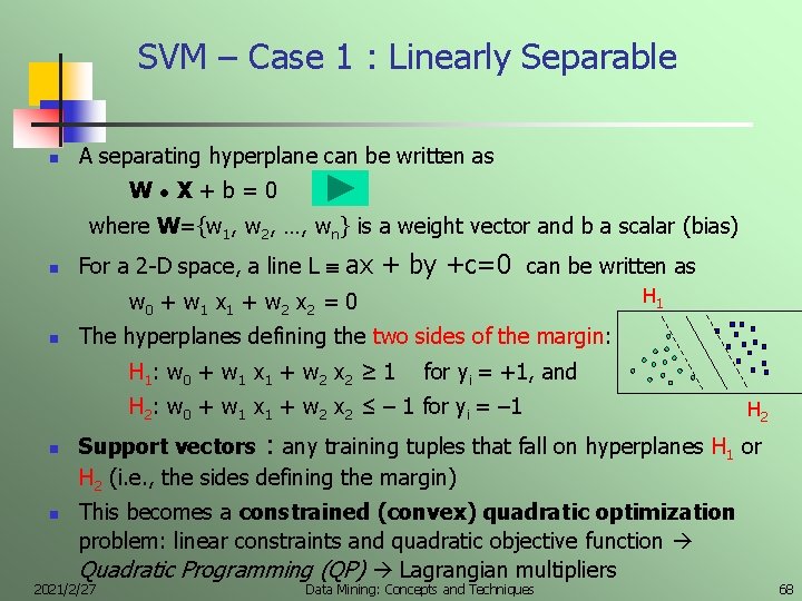
SVM – Case 1 : Linearly Separable n A separating hyperplane can be written as W ● X+b=0 where W={w 1, w 2, …, wn} is a weight vector and b a scalar (bias) n For a 2 -D space, a line L ax + by +c=0 can be written as H 1 w 0 + w 1 x 1 + w 2 x 2 = 0 n The hyperplanes defining the two sides of the margin: H 1 : w 0 + w 1 x 1 + w 2 x 2 ≥ 1 for yi = +1, and H 2: w 0 + w 1 x 1 + w 2 x 2 ≤ – 1 for yi = – 1 n n H 2 Support vectors : any training tuples that fall on hyperplanes H 1 or H 2 (i. e. , the sides defining the margin) This becomes a constrained (convex) quadratic optimization problem: linear constraints and quadratic objective function Quadratic Programming (QP) Lagrangian multipliers 2021/2/27 Data Mining: Concepts and Techniques 68

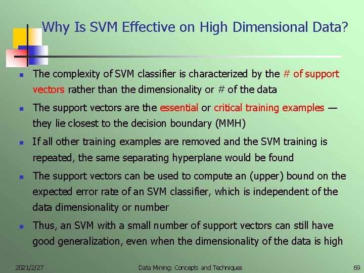
Why Is SVM Effective on High Dimensional Data? n The complexity of SVM classifier is characterized by the # of support vectors rather than the dimensionality or # of the data n The support vectors are the essential or critical training examples — they lie closest to the decision boundary (MMH) n If all other training examples are removed and the SVM training is repeated, the same separating hyperplane would be found n The support vectors can be used to compute an (upper) bound on the expected error rate of an SVM classifier, which is independent of the data dimensionality or number n Thus, an SVM with a small number of support vectors can still have good generalization, even when the dimensionality of the data is high 2021/2/27 Data Mining: Concepts and Techniques 69

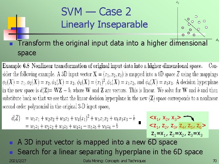
SVM — Case 2 Linearly Inseparable n Transform the original input data into a higher dimensional space <x 1, x 2, x 3> <z 1, z 2, z 3, z 4, z 5, z 6> z 1=x 1, z 2=x 2, z 3=x 3 n n A 3 D input vector is mapped into a new 6 D space Search for a linear separating hyperplane in the 6 D space 2021/2/27 Data Mining: Concepts and Techniques 70

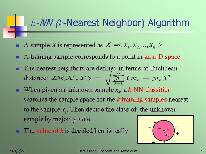
k-NN (k-Nearest Neighbor) Algorithm n A sample X is represented as n A training sample corresponds to a point in an n-D space. n n n The nearest neighbors are defined in terms of Euclidean distance: When given an unknown sample xq, a k-NN classifier searches the sample space for the k training samples nearest to the sample xq. Then decide the class of the unknown sample by majority vote. _ The value of k is decided heuristically. 2021/2/27 Data Mining: Concepts and Techniques _ _ _ + +. _ xq + _ + 71

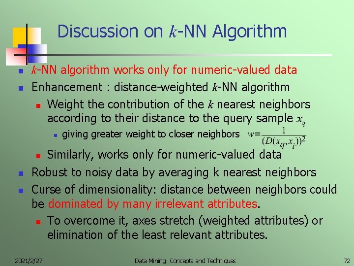
Discussion on k-NN Algorithm n n k-NN algorithm works only for numeric-valued data Enhancement : distance-weighted k-NN algorithm n Weight the contribution of the k nearest neighbors according to their distance to the query sample xq n n giving greater weight to closer neighbors Similarly, works only for numeric-valued data Robust to noisy data by averaging k nearest neighbors Curse of dimensionality: distance between neighbors could be dominated by many irrelevant attributes. n To overcome it, axes stretch (weighted attributes) or elimination of the least relevant attributes. 2021/2/27 Data Mining: Concepts and Techniques 72

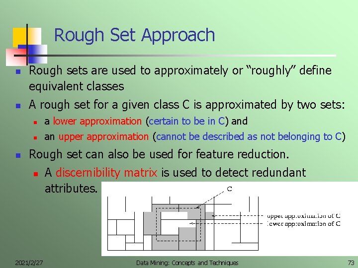
Rough Set Approach n n n Rough sets are used to approximately or “roughly” define equivalent classes A rough set for a given class C is approximated by two sets: n a lower approximation (certain to be in C) and n an upper approximation (cannot be described as not belonging to C) Rough set can also be used for feature reduction. n 2021/2/27 A discernibility matrix is used to detect redundant attributes. Data Mining: Concepts and Techniques 73

Fuzzy Set Approaches n Example Application : Credit approval n Credit Approval Rule : IF (years_employed >=2) AND (income >=50 K), THEN Credit = “approval” n Problem : What if a customer has had a job for at least two years and her income is $49 K ? n n Should she be approved or not ? Solution : Fuzzy set approaches IF (years_employed is medium) AND (income is high), THEN Credit is approval 2021/2/27 Data Mining: Concepts and Techniques 74

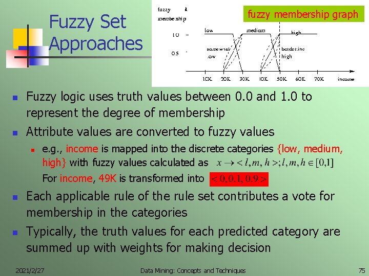
Fuzzy Set Approaches n n fuzzy membership graph Fuzzy logic uses truth values between 0. 0 and 1. 0 to represent the degree of membership Attribute values are converted to fuzzy values n e. g. , income is mapped into the discrete categories {low, medium, high} with fuzzy values calculated as For income, 49 K is transformed into n n Each applicable rule of the rule set contributes a vote for membership in the categories Typically, the truth values for each predicted category are summed up with weights for making decision 2021/2/27 Data Mining: Concepts and Techniques 75

Chapter 6 Classification and Prediction n n n n 2021/2/27 What is classification? What is prediction? Issues regarding classification and prediction Classification by decision tree induction Bayesian classification Classification by backpropagation Other classification methods Prediction Performance evaluation Summary Data Mining: Concepts and Techniques 76

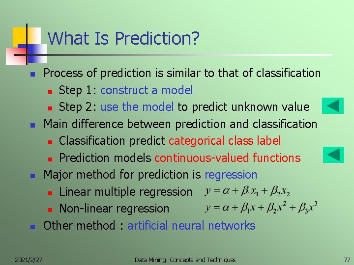
What Is Prediction? n n 2021/2/27 Process of prediction is similar to that of classification n Step 1: construct a model n Step 2: use the model to predict unknown value Main difference between prediction and classification n Classification predict categorical class label n Prediction models continuous-valued functions Major method for prediction is regression n Linear multiple regression n Non-linear regression Other method : artificial neural networks Data Mining: Concepts and Techniques 77

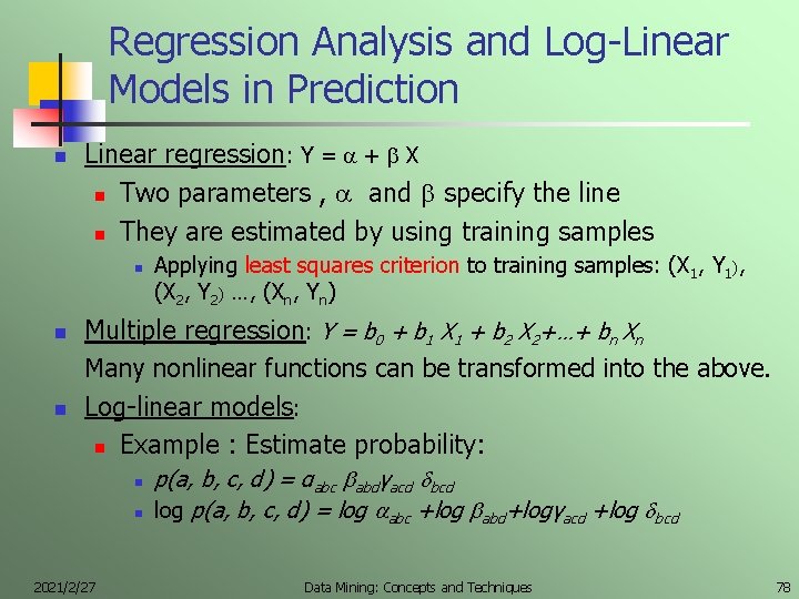
Regression Analysis and Log-Linear Models in Prediction n Linear regression: Y = + X n Two parameters , and specify the line n They are estimated by using training samples n n n Applying least squares criterion to training samples: (X 1, Y 1), (X 2, Y 2) …, (Xn, Yn) Multiple regression: Y = b 0 + b 1 X 1 + b 2 X 2+…+ bn Xn Many nonlinear functions can be transformed into the above. Log-linear models: n Example : Estimate probability: n n 2021/2/27 p(a, b, c, d) = αabc abdγacd bcd log p(a, b, c, d) = log abc +log abd+logγacd +log bcd Data Mining: Concepts and Techniques 78

Chapter 6 Classification and Prediction n n 2021/2/27 What is classification? What is prediction? Issues regarding classification and prediction Classification by decision tree induction Bayesian Classification by backpropagation Classification based on concepts from association rule mining Other classification methods Prediction Performance evaluation Summary Data Mining: Concepts and Techniques 79

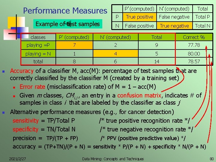
Performance Measures Example of test samples n n P’ (computed) N’ (computed) Total P True positive False negative Total P N False positive True negative Total N classes P’ (computed) N’ (computed) Total Correct % playing =P 7 2 9 77. 78 playing = N 1 4 5 80. 00 total 8 6 14 78. 57 Accuracy of a classifier M, acc(M): percentage of test samples that are correctly classified by the classifier M (created by a training set) n Error rate (misclassification rate) of M = 1 – acc(M) n Given m classes, CMi, j , an entry in a confusion matrix, indicates # of samples in class i that are labeled by the classifier as class j Alternative performance measures (e. g. , for cancer detection) sensitivity = TP/Total P /* true positive recognition rate */ specificity = TN/Total N /* true negative recognition rate */ precision = TP/(TP + FP) /* PPV (positive predictive value) */ accuracy = (TP+TN)/(P + N) = sensitivity * P/(P + N) + specificity * N/(P + N) 2021/2/27 Data Mining: Concepts and Techniques 80

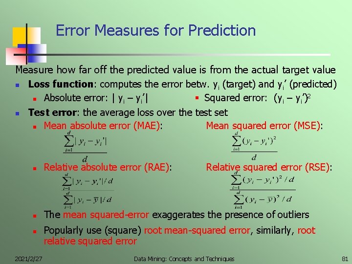
Error Measures for Prediction Measure how far off the predicted value is from the actual target value n Loss function: computes the error betw. yi (target) and yi’ (predicted) n Absolute error: | yi – yi’| Squared error: (yi – yi’)2 n Test error: the average loss over the test set n Mean absolute error (MAE): Mean squared error (MSE): n Relative absolute error (RAE): n The mean squared-error exaggerates the presence of outliers n 2021/2/27 Relative squared error (RSE): Popularly use (square) root mean-squared error, similarly, root relative squared error Data Mining: Concepts and Techniques 81

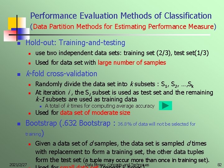
Performance Evaluation Methods of Classification (Data Partition Methods for Estimating Performance Measure) n n Hold-out: Training-and-testing n use two independent data sets: training set (2/3), test set(1/3) n Used for data set with large number of samples k-fold cross-validation n n Randomly divide the data set into k subsets : S 1, S 2, …, Sk At iteration i , the Si subset is used as test set and the remaining k-1 subsets are used as training data n n n A total of k times for computing average accuracy Used for data set of moderate size Bootstrap (. 632 Bootstrap : training) n 2021/2/27 36. 8% of data will not be selected for Given a data set of d samples, the data set is sampled d times with replacement to form a training set, the other data tuples form the test set (a tuple may occur more than once in training set). Data Mining: Concepts and Techniques 82

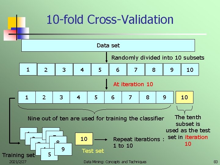
10 -fold Cross-Validation Data set Randomly divided into 10 subsets 1 2 3 4 5 6 7 8 9 10 At iteration 10 1 2 3 4 5 6 7 8 9 10 The tenth subset is used as the test Repeat iterations : set in iteration 10 1 to 10 Nine out of ten are used for training the classifier 1 2 Training set 2021/2/27 3 6 7 8 4 5 10 9 Test set Data Mining: Concepts and Techniques 83

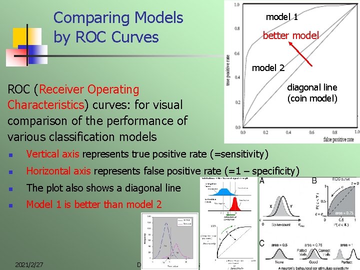
Comparing Models by ROC Curves model 1 better model 2 ROC (Receiver Operating Characteristics) curves: for visual comparison of the performance of various classification models diagonal line (coin model) n Vertical axis represents true positive rate (=sensitivity) n Horizontal axis represents false positive rate (=1 – specificity) n The plot also shows a diagonal line n Model 1 is better than model 2 2021/2/27 Data Mining: Concepts and Techniques 84

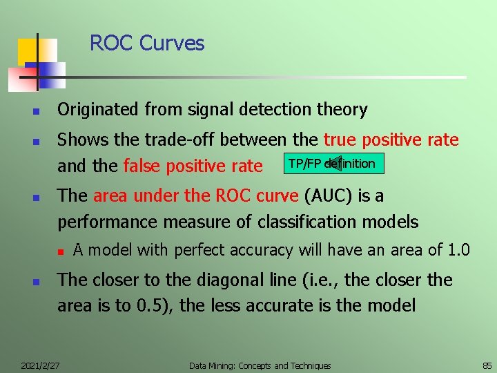
ROC Curves n n n Originated from signal detection theory Shows the trade-off between the true positive rate and the false positive rate TP/FP definition The area under the ROC curve (AUC) is a performance measure of classification models n n A model with perfect accuracy will have an area of 1. 0 The closer to the diagonal line (i. e. , the closer the area is to 0. 5), the less accurate is the model 2021/2/27 Data Mining: Concepts and Techniques 85

Chapter 6 Classification and Prediction n n 2021/2/27 What is classification? What is prediction? Issues regarding classification and prediction Classification by decision tree induction Bayesian Classification by backpropagation Classification based on concepts from association rule mining Other Classification Methods Prediction Estimating classification accuracy Summary Data Mining: Concepts and Techniques 86

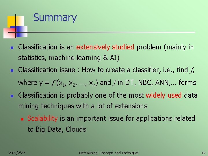
Summary n Classification is an extensively studied problem (mainly in statistics, machine learning & AI) n Classification issue : How to create a classifier, i. e. , find f, where y = f (x 1, x 2, …, xn) and f in DT, NBC, ANN, … forms n Classification is probably one of the most widely used data mining techniques with a lot of extensions n Scalability is an important issue for applications related to Big Data, Clouds 2021/2/27 Data Mining: Concepts and Techniques 87