Classification and Diagnostic of Cancers Classification and diagnostic

Classification and Diagnostic of Cancers Classification and diagnostic prediction of cancers using gene expression profiling and artificial neural networks JAVED KHAN ET AL. NATURE MEDICINE – Volume 7 – Number 6 – JUNE 2001 Aronashvili Reuven

Overview n The purpose of this study was to develop a method of classifying cancers to specific diagnostic categories based on their gene expression signatures using artificial neural networks (ANNs). n We trained the ANNs using the small, round blue-cell tumors (SRBCTs) as a model.

The SRBCTs Ø The small, round blue cell tumors (SRBCTs) of childhood(four distinct categories): 1. Neuroblastoma (NB) 2. Rhabdomyosarcoma (RMS) 3. Non-Hodgkin lymphoma (NHL) – (BL) 4. Ewing family of tumors (EWS) Ø Often present diagnostic dilemmas in clinical practice because they are similar in appearance on routine histology. However accurate diagnosis is essential – as treatment options , response to therapy, etc, vary. No single test can precisely distinguish SRBCTs – Immunohistochemistry, cytogenetics, interphase fluorescent in situ hybridization and reverse transcription. Ø Ø

Introduction

Artificial Neural Networks ANNs

Artificial Neural Networks (ANNs) – put to the task. n n Modeled on the structure and behavior of neurons in the human brain. Can be trained to recognize and categorize complex patterns. Pattern recognition achieved by adjusting of the ANN by a process of error minimization through learning from experience. ANNs were applied to decipher gene-expression signatures of SRBCTs and then used for diagnostic classification.

Principal Component Analysis PCA

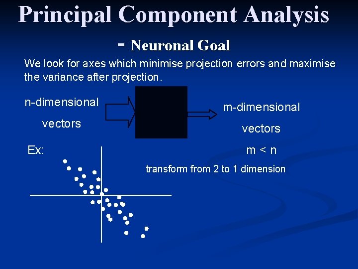
Principal Component Analysis - Neuronal Goal We look for axes which minimise projection errors and maximise the variance after projection. n-dimensional m-dimensional vectors Ex: m<n transform from 2 to 1 dimension

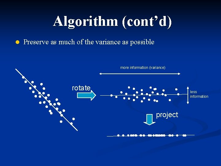
Algorithm (cont’d) l Preserve as much of the variance as possible more information (variance) rotate less information project

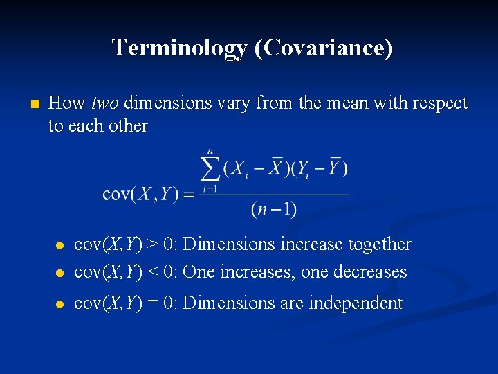
Terminology (Covariance) n How two dimensions vary from the mean with respect to each other l cov(X, Y) > 0: Dimensions increase together cov(X, Y) < 0: One increases, one decreases l cov(X, Y) = 0: Dimensions are independent l

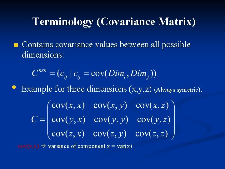
Terminology (Covariance Matrix) n • Contains covariance values between all possible dimensions: Example for three dimensions (x, y, z) (Always symetric): cov(x, x) variance of component x = var(x)

Properties of the Cov matrix n Can be used for creating a distance that is not sensitive to linear transformation n Can be used to find directions which maximize the variance n Determines a Gaussian distribution uniquely (up to a shift)

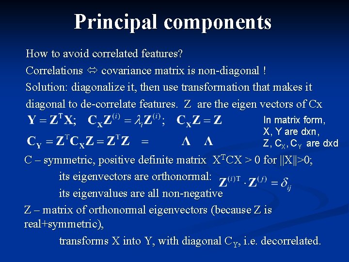
Principal components How to avoid correlated features? Correlations covariance matrix is non-diagonal ! Solution: diagonalize it, then use transformation that makes it diagonal to de-correlate features. Z are the eigen vectors of Cx In matrix form, X, Y are dxn, Z, CX, CY are dxd C – symmetric, positive definite matrix XTCX > 0 for ||X||>0; its eigenvectors are orthonormal: its eigenvalues are all non-negative Z – matrix of orthonormal eigenvectors (because Z is real+symmetric), transforms X into Y, with diagonal CY, i. e. decorrelated.

Matrix form Eigen problem for C matrix in matrix form:

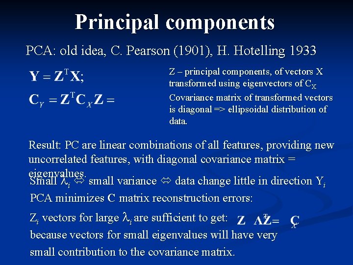
Principal components PCA: old idea, C. Pearson (1901), H. Hotelling 1933 Z – principal components, of vectors X transformed using eigenvectors of CX Covariance matrix of transformed vectors is diagonal => ellipsoidal distribution of data. Result: PC are linear combinations of all features, providing new uncorrelated features, with diagonal covariance matrix = eigenvalues. Small li small variance data change little in direction Yi PCA minimizes C matrix reconstruction errors: Zi vectors for large li are sufficient to get: because vectors for small eigenvalues will have very small contribution to the covariance matrix.

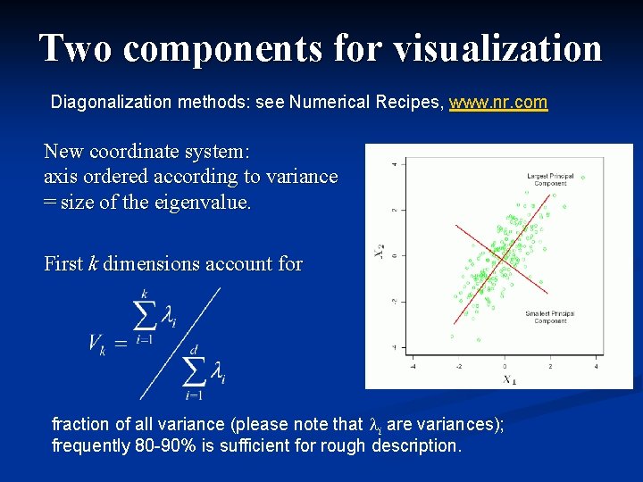
Two components for visualization Diagonalization methods: see Numerical Recipes, www. nr. com New coordinate system: axis ordered according to variance = size of the eigenvalue. First k dimensions account for fraction of all variance (please note that li are variances); frequently 80 -90% is sufficient for rough description.

PCA properties PC Analysis (PCA) may be achieved by: n transformation making covariance matrix diagonal n projecting the data on a line for which the sums of squares of distances from original points to projections is minimal. n orthogonal transformation to new variables that have stationary variances True covariance matrices are usually not known, estimated from data. This works well on single-cluster data; more complex structure may require local PCA, separately for each cluster. PC is useful for: finding new, more informative, uncorrelated features; reducing dimensionality: reject low variance features, reconstructing covariance matrices from low-dim data.

PCA disadvantages Useful for dimensionality reduction but: Largest variance determines which components are used, but does not guarantee interesting viewpoint for clustering data. n The meaning of features is lost when linear combinations are formed. Analysis of coefficients in Z 1 and other important eigenvectors may show which original features are given much weight. n PCA may be also done in an efficient way by performing singular value decomposition of the standardized data matrix. PCA is also called Karhuen-Loève transformation. Many variants of PCA are described in A. Webb, Statistical pattern recognition, J. Wiley 2002.

Next Summed Square Error

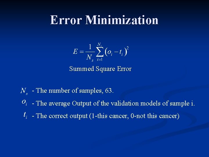
Error Minimization Summed Square Error - The number of samples, 63. - The average Output of the validation models of sample i. - The correct output (1 -this cancer, 0 -not this cancer)

The Algorithm

Calibration and validation of the ANN Models. n The gene expression values are taken from c. DNA microarrays containing 6567 genes. n 63 training samples comprised of 13 EWS and 10 RMS from tumor biopsy and 10 EWS, 10 RMS, 12 NB, 8 BL from cell lines. n 25 test samples comprised of 5 EWS, 5 RMS, 4 NB, from tumors and 1 EWS, 2 NB, 3 BL from cell lines. Plus 5 non-SRBCT samples (to test ability of reject diagnosis).

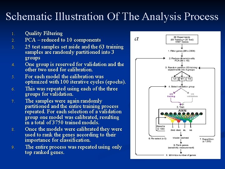
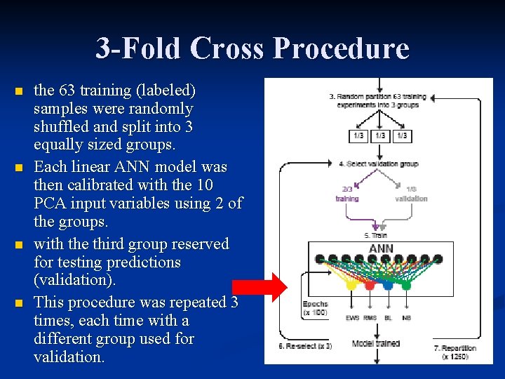
Schematic Illustration Of The Analysis Process 1. 2. 3. 4. 5. 6. 7. 8. 9. Quality Filtering PCA – reduced to 10 components 25 test samples set aside and the 63 training samples are randomly partitioned into 3 groups One group is reserved for validation and the other two used for calibration. For each model the calibration was optimized with 100 iterative cycles (epochs). This was repeated using each of the three groups for validation. The samples were again randomly partitioned and the entire training process repeated. For each selection of a validation group one model was calibrated, resulting in a total of 3750 trained models. Once the models were calibrated they were used to rank the genes according to their importance for classification. The entire process was repeated using only top ranked genes.

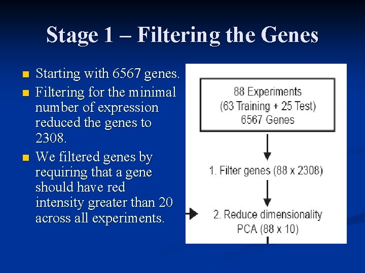
Stage 1 – Filtering the Genes n n n Starting with 6567 genes. Filtering for the minimal number of expression reduced the genes to 2308. We filtered genes by requiring that a gene should have red intensity greater than 20 across all experiments.

Cont. n n 10 dominant PCA components per sample were used as inputs. (contained 63% of the variance in the data matrix. ) The remaining PCA components contained variance unrelated to separating the four cancers. n So we have 88 x 10 inputs. (88 samples with their 10 PCA components). n Four outputs – (EWS, RMS, NB, BL).

3 -Fold Cross Procedure n n the 63 training (labeled) samples were randomly shuffled and split into 3 equally sized groups. Each linear ANN model was then calibrated with the 10 PCA input variables using 2 of the groups. with the third group reserved for testing predictions (validation). This procedure was repeated 3 times, each time with a different group used for validation.

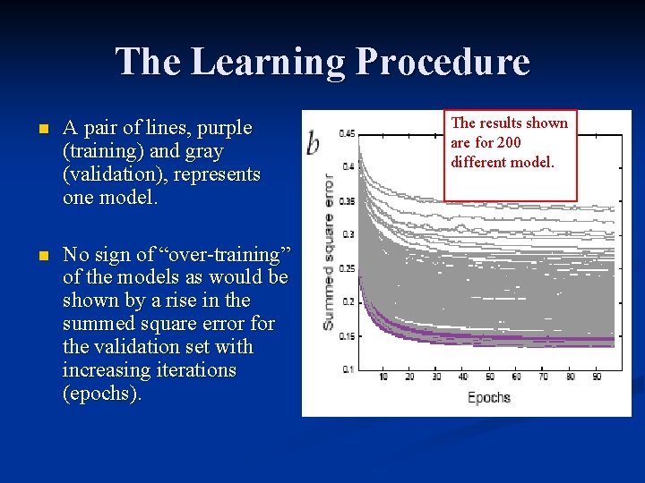
The Learning Procedure n A pair of lines, purple (training) and gray (validation), represents one model. n No sign of “over-training” of the models as would be shown by a rise in the summed square error for the validation set with increasing iterations (epochs). The results shown are for 200 different model.

Cont. Validation n The random shuffling was redone 1250 times (for each shuffling 3 ANN models). Thus, in total, each sample belonged to a validation set 1250 times, and 3750 ANN models were calibrated. n Each ANN model gives a number between 0 (not this cancer type) and 1(this cancer type) as an output for each cancer type. The average for all model outputs for every validation sample is then computed (denoted the average committee vote). Each sample is classified as belonging to the cancer type corresponding to the largest committee vote. n n

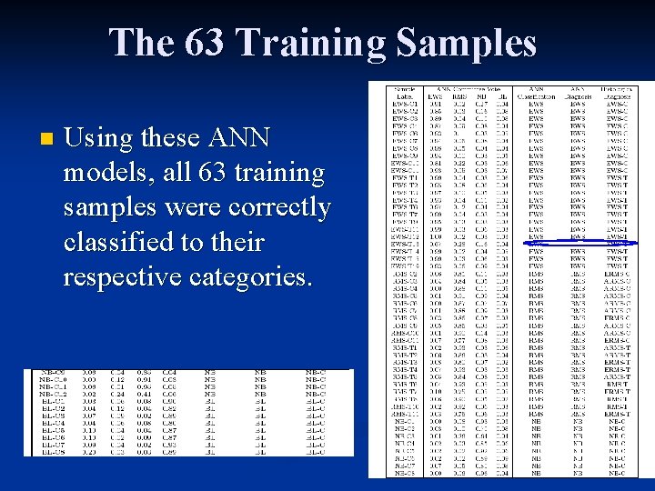
The 63 Training Samples n Using these ANN models, all 63 training samples were correctly classified to their respective categories.

Optimization of Genes used for Classification. The contribution of each gene to the classification by the ANN models was then assessed. n Feature extraction was performed in a model dependent way due to relatively few samples. n This was achieved by monitoring the sensitivity of classification to a change in the expression level of each gene, using the 3750 previously calibrated models. n

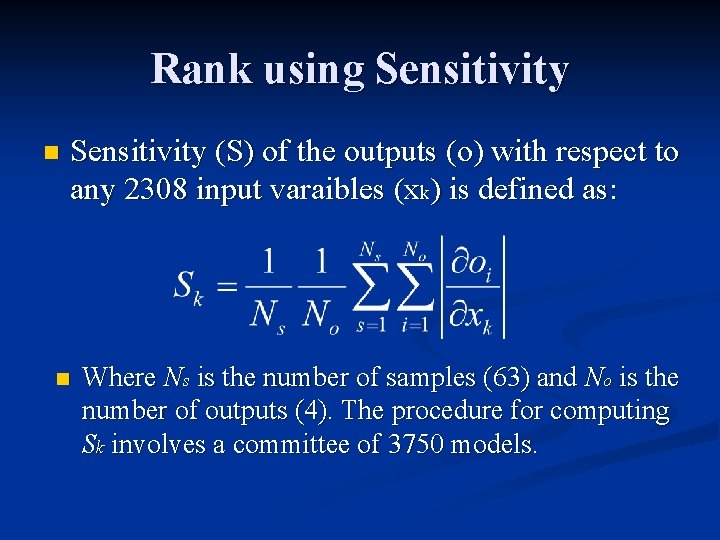
Rank using Sensitivity n Sensitivity (S) of the outputs (o) with respect to any 2308 input varaibles (xk) is defined as: n Where Ns is the number of samples (63) and No is the number of outputs (4). The procedure for computing Sk involves a committee of 3750 models.

Cont. n In this way genes were ranked according to the significance of classification and the classification error rate using increasing numbers of these ranked genes was determined.

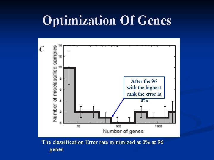
Optimization Of Genes After the 96 with the highest rank the error is 0% The classification Error rate minimized at 0% at 96 genes

Recalibration The entire process (2– 7) was repeated using only the 96 top ranked genes (9). n The 10 dominant PCA components for these 96 genes contained 79% of the variance in the data matrix. n Using only these 96 genes, we recalibrated the ANN models. n Again correctly classified all 63 samples. n

Assessing the Quality of Classification - Diagnoses. n The aim of diagnoses is to be able to reject test samples which do not belong to any of the four categories. n To do this a distance dc from a sample to the ideal vote for each cancer type was calculated:

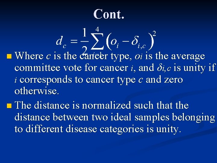
Cont. n Where c is the cancer type, oi is the average committee vote for cancer i, and δi, c is unity if i corresponds to cancer type c and zero otherwise. n The distance is normalized such that the distance between two ideal samples belonging to different disease categories is unity.

Cont. n Based on the validation set, an empirical probability distribution of distances for each cancer type was generated. n The empirical probability distributions are built using each ANN model independently. n Thus, the number of entries in each distribution is given by 1250 multiplied with the number of samples belonging to the caner type.

Cont. n n For a given test sample it is thus possible to reject possible classifications based on these probability distributions. Hence for each disease category a cutoff distance from the ideal sample was defined within which it is expected a sample of this category to fall in. The distance given by the 95 th percentile of the probability distribution was chosen. This is the basis of diagnoses, as a sample that falls outside the cutoff distance cannot be confidently diagnosed.

Cont. n If a sample falls outside the 95 th percentile of the probability distribution of distances between samples and their ideal output (for example for EWS it is EWS = 1, RMS = NB = BL = 0), its diagnosis is rejected. n Using the 3750 ANN models calibrated with the 96 genes all of the 5 non-SRBCT samples were excluded from any of the four diagnostic categories, since they fell outside the 95 percentile.

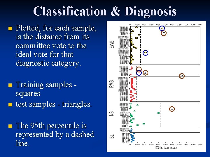
Classification & Diagnosis n Plotted, for each sample, is the distance from its committee vote to the ideal vote for that diagnostic category. n Training samples squares test samples - triangles. n n The 95 th percentile is represented by a dashed line.

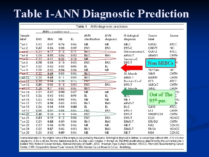
Table 1 -ANN Diagnostic Prediction b b b b Non SRBCs Out of The 95 th per.

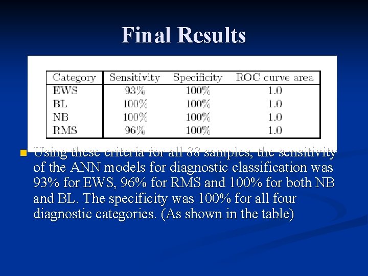
Final Results n Using these criteria for all 88 samples, the sensitivity of the ANN models for diagnostic classification was 93% for EWS, 96% for RMS and 100% for both NB and BL. The specificity was 100% for all four diagnostic categories. (As shown in the table)

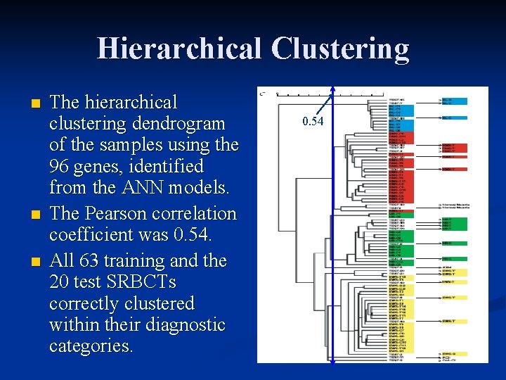
Hierarchical Clustering Using The 96 Top Ranked Genes

Hierarchical Clustering n n n The hierarchical clustering dendrogram of the samples using the 96 genes, identified from the ANN models. The Pearson correlation coefficient was 0. 54. All 63 training and the 20 test SRBCTs correctly clustered within their diagnostic categories. 0. 54

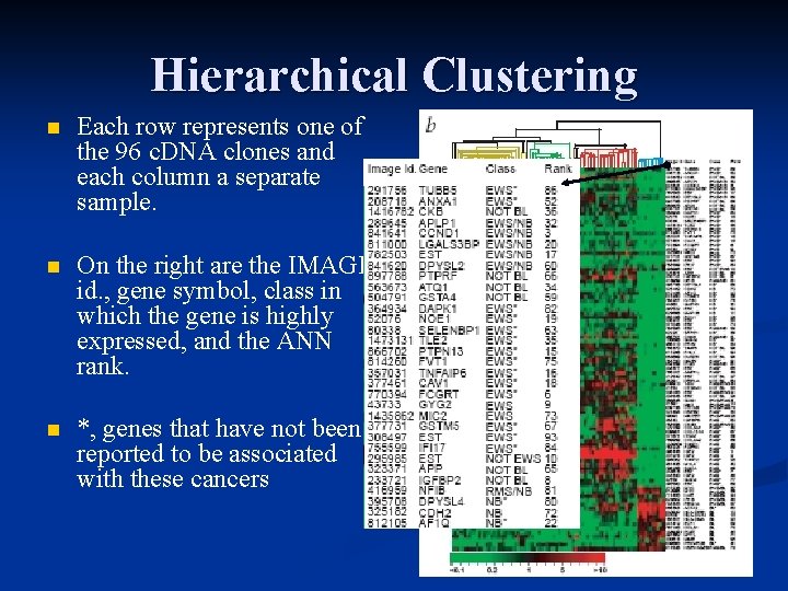
Hierarchical Clustering n Each row represents one of the 96 c. DNA clones and each column a separate sample. n On the right are the IMAGE id. , gene symbol, class in which the gene is highly expressed, and the ANN rank. n *, genes that have not been reported to be associated with these cancers

Conclusions n When we tested the ANN models calibrated using the 96 genes on 25 blinded samples, we were able to correctly classify all 20 samples of SRBCTs and reject the 5 non-SRBCTs. This supports the potential use of these methods as an adjunct to routine histological diagnosis.

Conclusions n Although we achieved high sensitivity and specificity for diagnostic classification, we believe that with larger arrays and more samples it will be possible to improve on the sensitivity of these models for purposes of diagnosis in clinical practice.

Questions?