Classification Algorithms Linear Regression Decision Tree Induction Bayes

Classification Algorithms Linear Regression Decision Tree Induction Bayes Classification Methods Rule-Based Classification Model Evaluation and Selection Techniques to Improve Classification Accuracy: Ensemble Methods Summary 1

Supervised vs. Unsupervised Learning Supervised learning (classification) Supervision: The training data (observations, measurements, etc. ) are accompanied by labels indicating the class of the observations New data is classified based on the training set Unsupervised learning (clustering) The class labels are unknown Given a set of measurements, observations, etc. with the aim of establishing the existence of classes or clusters in the data 2

Prediction Problems: Classification vs. Numeric Prediction Classification predicts categorical class labels (discrete or nominal) classifies data (constructs a model) based on the training set and the values (class labels) in a classifying attribute and uses it in classifying new data Numeric Prediction models continuous-valued functions, i. e. , predicts unknown or missing values 3

Classification—A Two-Step Process Model construction: describing a set of predetermined classes Each tuple/sample is assumed to belong to a predefined class, as determined by the class label attribute The set of tuples used for model construction is training set The model is represented as classification rules, decision trees, or mathematical formulae Model usage: for classifying future or unknown objects Estimate accuracy of the model The known label of test sample is compared with the classified result from the model Accuracy rate is the percentage of test set samples that are correctly classified by the model Test set is independent of training set (otherwise overfitting) If the accuracy is acceptable, use the model to classify new data Note: If the test set is used to select models, it is called validation (test) set 4

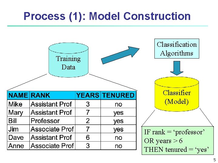
Process (1): Model Construction Training Data Classification Algorithms Classifier (Model) IF rank = ‘professor’ OR years > 6 THEN tenured = ‘yes’ 5

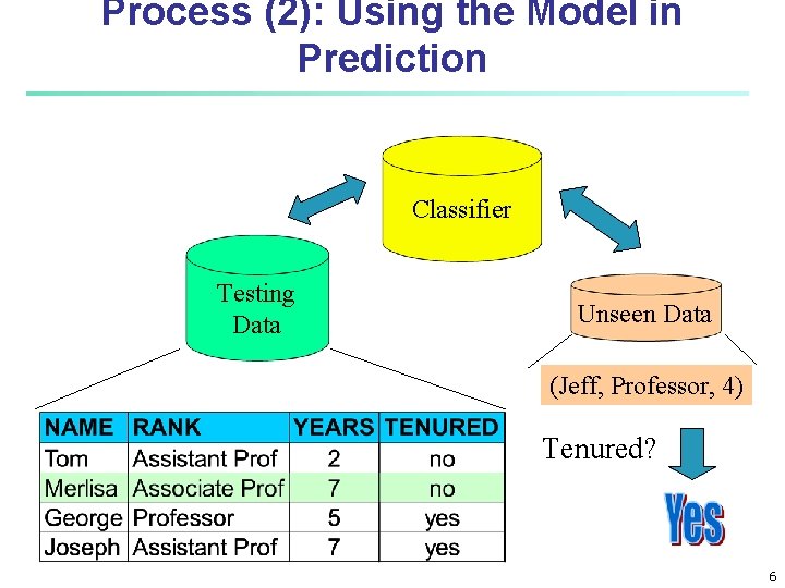
Process (2): Using the Model in Prediction Classifier Testing Data Unseen Data (Jeff, Professor, 4) Tenured? 6

Chapter 8. Classification: Basic Concepts Decision Tree Induction Bayes Classification Methods Rule-Based Classification Model Evaluation and Selection Techniques to Improve Classification Accuracy: Ensemble Methods Summary 7

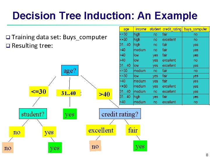
Decision Tree Induction: An Example Training data set: Buys_computer Resulting tree: age? <=30 31. . 40 overcast student? no no >40 credit rating? yes yes excellent no fair yes 8

Algorithm for Decision Tree Induction Basic algorithm (a greedy algorithm) Tree is constructed in a top-down recursive divide-and-conquer manner At start, all the training examples are at the root Attributes are categorical (if continuous-valued, they are discretized in advance) Examples are Examples partitioned recursively based on selected attributes Test attributes are selected on the basis of a heuristic or statistical measure (e. g. , information gain) Conditions for stopping partitioning All samples for a given node belong to the same class There are no remaining attributes for further partitioning There are no samples left 9

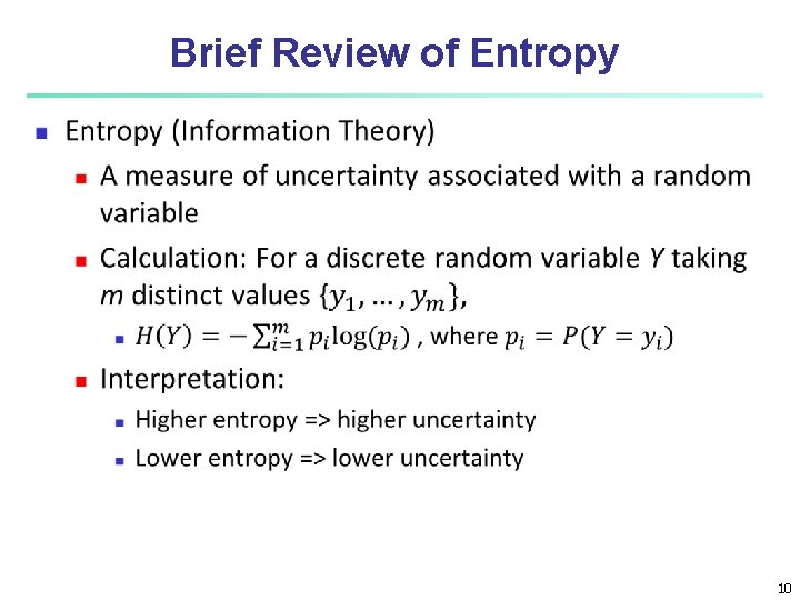
Brief Review of Entropy 10

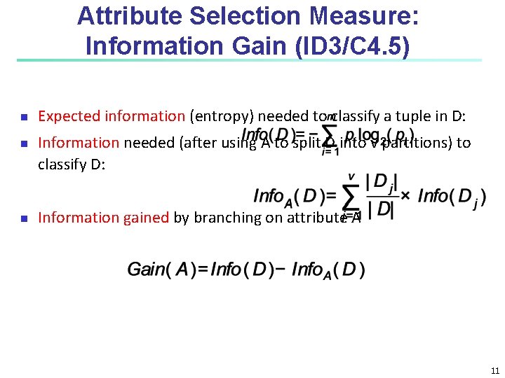
Attribute Selection Measure: Information Gain (ID 3/C 4. 5) Expected information (entropy) needed to classify a tuple in D: Information needed (after using A to split D into v partitions) to classify D: Information gained by branching on attribute A 11

Attribute Selection Measure: Information Gain (ID 3/C 4. 5) Expected information (entropy) needed to classify a tuple in D: Information needed (after using A to split D into v partitions) to classify D: Information gained by branching on attribute A 12

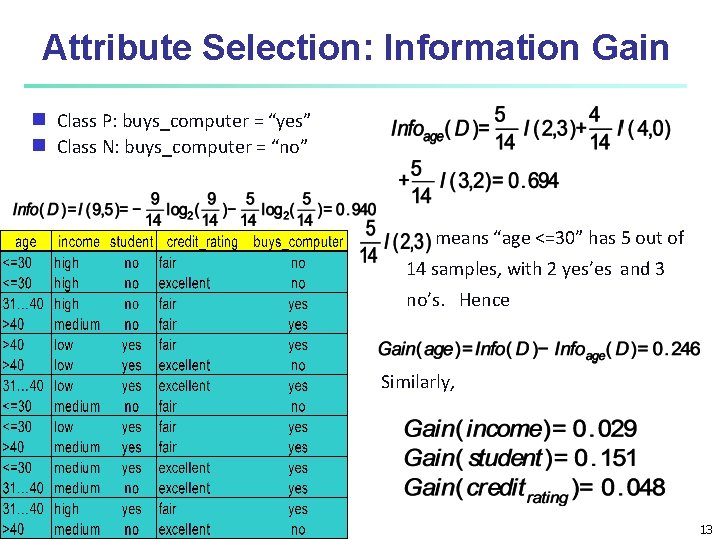
Attribute Selection: Information Gain Class P: buys_computer = “yes” Class N: buys_computer = “no” means “age <=30” has 5 out of 14 samples, with 2 yes’es and 3 no’s. Hence Similarly, 13

Overfitting and Tree Pruning Overfitting: An induced tree may overfit the training data Too many branches, some may reflect anomalies due to noise or outliers Poor accuracy for unseen samples Two approaches to avoid overfitting Prepruning: Halt tree construction early do not split a node if this would result in the goodness measure falling below a threshold Difficult to choose an appropriate threshold Postpruning: Remove branches from a “fully grown” tree—get a sequence of progressively pruned trees Use a set of data different from the training data to decide which is the “best pruned tree” 14

Chapter 8. Classification: Basic Concepts Decision Tree Induction Bayes Classification Methods Rule-Based Classification Model Evaluation and Selection Techniques to Improve Classification Accuracy: Ensemble Methods Summary 15

Bayesian Classification: Why? A statistical classifier: performs probabilistic prediction, i. e. , predicts class membership probabilities Foundation: Based on Bayes’ Theorem. Performance: A simple Bayesian classifier, naïve Bayesian classifier, has comparable performance with decision tree and selected neural network classifiers Incremental: Each training example can incrementally increase/decrease the probability that a hypothesis is correct — prior knowledge can be combined with observed data Standard: Even when Bayesian methods are computationally intractable, they can provide a standard of optimal decision making against which other methods can be measured 16

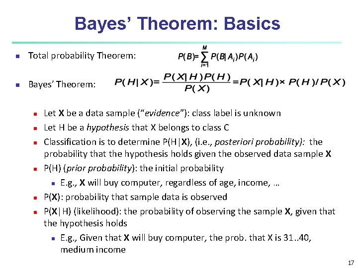
Bayes’ Theorem: Basics Total probability Theorem: Bayes’ Theorem: Let X be a data sample (“evidence”): class label is unknown Let H be a hypothesis that X belongs to class C Classification is to determine P(H|X), (i. e. , posteriori probability): the probability that the hypothesis holds given the observed data sample X P(H) (prior probability): the initial probability E. g. , X will buy computer, regardless of age, income, … P(X): probability that sample data is observed P(X|H) (likelihood): the probability of observing the sample X, given that the hypothesis holds E. g. , Given that X will buy computer, the prob. that X is 31. . 40, medium income 17

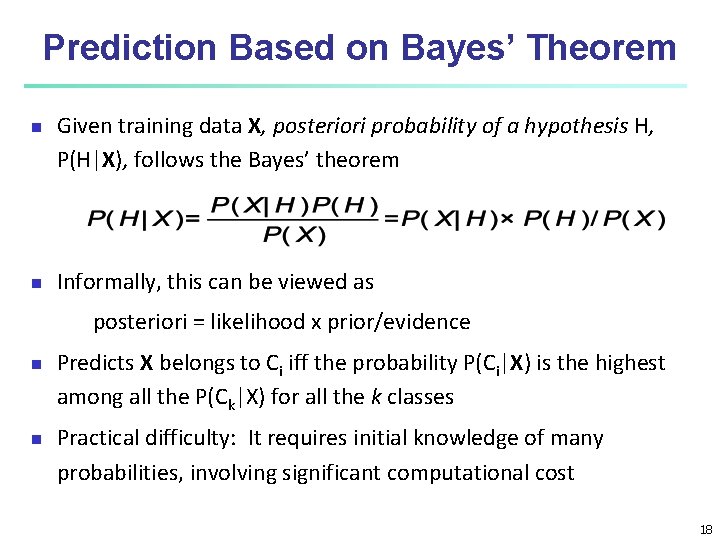
Prediction Based on Bayes’ Theorem Given training data X, posteriori probability of a hypothesis H, P(H|X), follows the Bayes’ theorem Informally, this can be viewed as posteriori = likelihood x prior/evidence Predicts X belongs to Ci iff the probability P(Ci|X) is the highest among all the P(Ck|X) for all the k classes Practical difficulty: It requires initial knowledge of many probabilities, involving significant computational cost 18

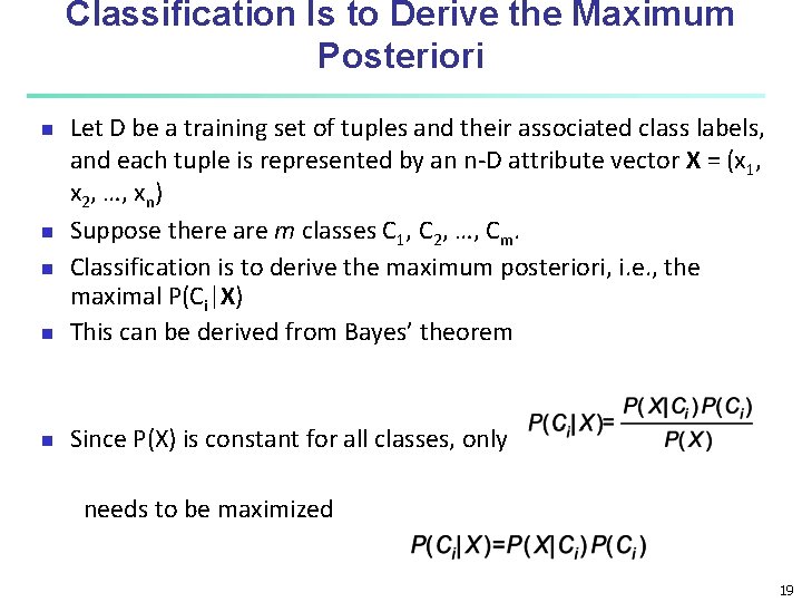
Classification Is to Derive the Maximum Posteriori Let D be a training set of tuples and their associated class labels, and each tuple is represented by an n-D attribute vector X = (x 1, x 2, …, xn) Suppose there are m classes C 1, C 2, …, Cm. Classification is to derive the maximum posteriori, i. e. , the maximal P(Ci|X) This can be derived from Bayes’ theorem Since P(X) is constant for all classes, only needs to be maximized 19

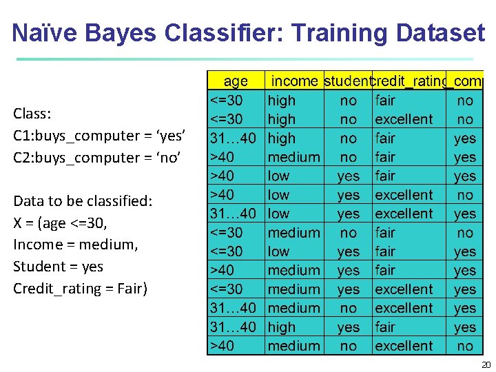
Naïve Bayes Classifier: Training Dataset Class: C 1: buys_computer = ‘yes’ C 2: buys_computer = ‘no’ Data to be classified: X = (age <=30, Income = medium, Student = yes Credit_rating = Fair) 20

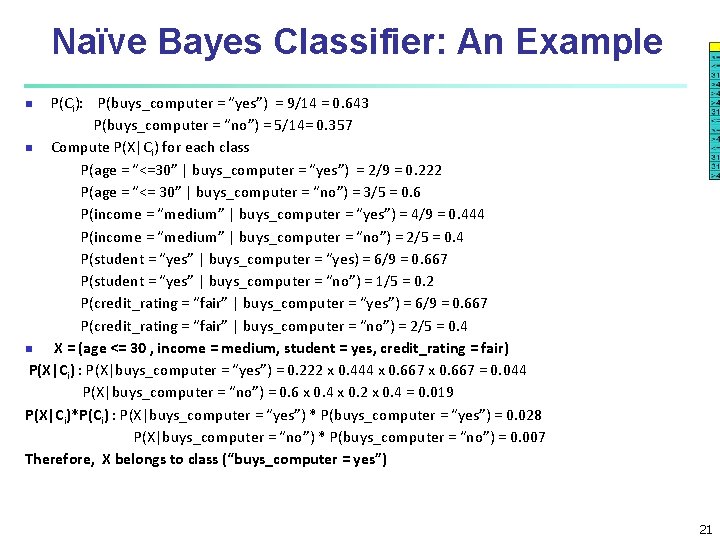
Naïve Bayes Classifier: An Example P(Ci): P(buys_computer = “yes”) = 9/14 = 0. 643 P(buys_computer = “no”) = 5/14= 0. 357 Compute P(X|Ci) for each class P(age = “<=30” | buys_computer = “yes”) = 2/9 = 0. 222 P(age = “<= 30” | buys_computer = “no”) = 3/5 = 0. 6 P(income = “medium” | buys_computer = “yes”) = 4/9 = 0. 444 P(income = “medium” | buys_computer = “no”) = 2/5 = 0. 4 P(student = “yes” | buys_computer = “yes) = 6/9 = 0. 667 P(student = “yes” | buys_computer = “no”) = 1/5 = 0. 2 P(credit_rating = “fair” | buys_computer = “yes”) = 6/9 = 0. 667 P(credit_rating = “fair” | buys_computer = “no”) = 2/5 = 0. 4 X = (age <= 30 , income = medium, student = yes, credit_rating = fair) P(X|Ci) : P(X|buys_computer = “yes”) = 0. 222 x 0. 444 x 0. 667 = 0. 044 P(X|buys_computer = “no”) = 0. 6 x 0. 4 x 0. 2 x 0. 4 = 0. 019 P(X|Ci)*P(Ci) : P(X|buys_computer = “yes”) * P(buys_computer = “yes”) = 0. 028 P(X|buys_computer = “no”) * P(buys_computer = “no”) = 0. 007 Therefore, X belongs to class (“buys_computer = yes”) 21

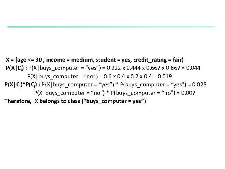
X = (age <= 30 , income = medium, student = yes, credit_rating = fair) P(X|Ci) : P(X|buys_computer = “yes”) = 0. 222 x 0. 444 x 0. 667 = 0. 044 P(X|buys_computer = “no”) = 0. 6 x 0. 4 x 0. 2 x 0. 4 = 0. 019 P(X|Ci)*P(Ci) : P(X|buys_computer = “yes”) * P(buys_computer = “yes”) = 0. 028 P(X|buys_computer = “no”) * P(buys_computer = “no”) = 0. 007 Therefore, X belongs to class (“buys_computer = yes”)

Comparison of Decision Tree and Baysian Classification 23