Classification Algorithms Continued Outline Rules Linear Models Regression

Classification Algorithms – Continued

Outline § Rules § Linear Models (Regression) § Instance-based (Nearest-neighbor) 2

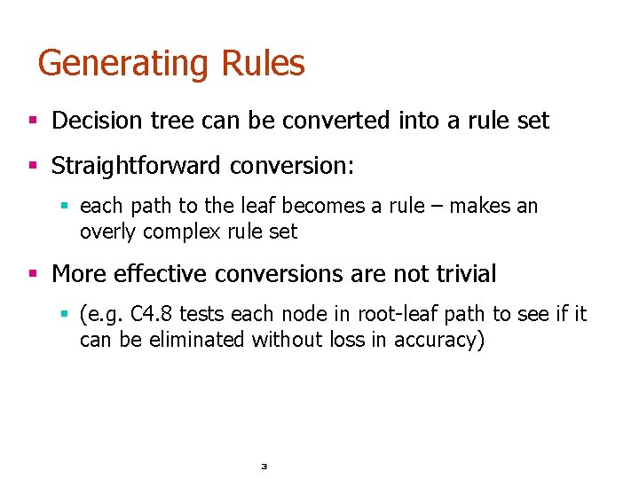
Generating Rules § Decision tree can be converted into a rule set § Straightforward conversion: § each path to the leaf becomes a rule – makes an overly complex rule set § More effective conversions are not trivial § (e. g. C 4. 8 tests each node in root-leaf path to see if it can be eliminated without loss in accuracy) 3

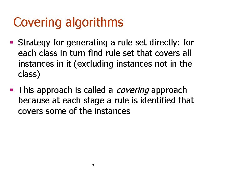
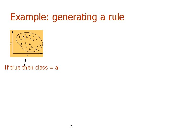
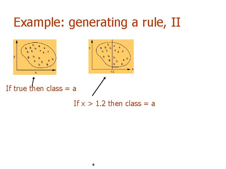
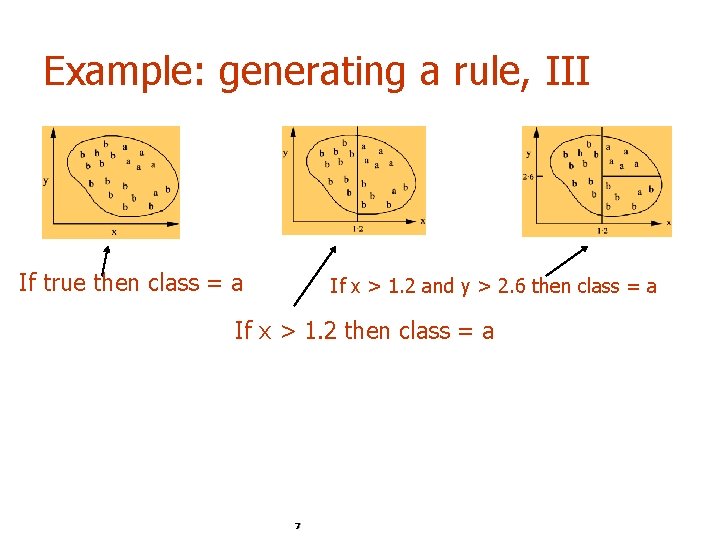
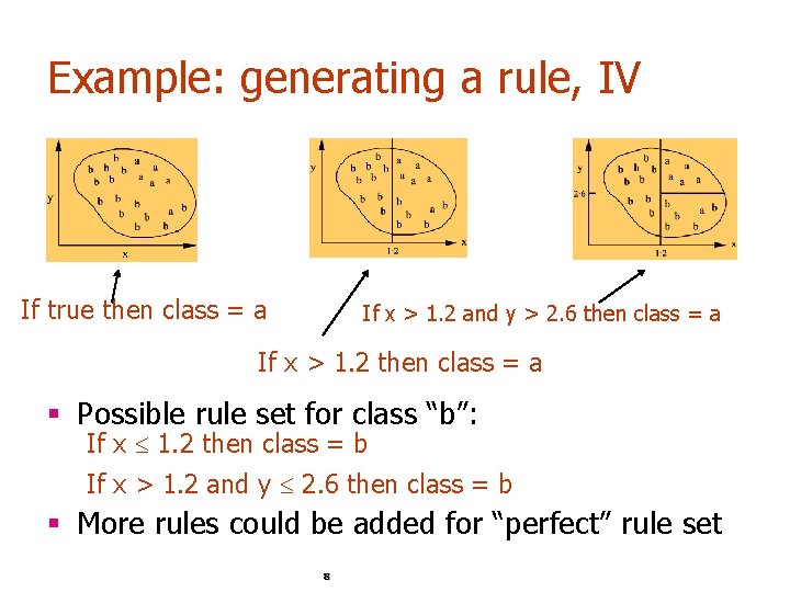
Covering algorithms § Strategy for generating a rule set directly: for each class in turn find rule set that covers all instances in it (excluding instances not in the class) § This approach is called a covering approach because at each stage a rule is identified that covers some of the instances 4

Example: generating a rule If true then class = a 5

Example: generating a rule, II If true then class = a If x > 1. 2 then class = a 6

Example: generating a rule, III If true then class = a If x > 1. 2 and y > 2. 6 then class = a If x > 1. 2 then class = a 7

Example: generating a rule, IV If true then class = a If x > 1. 2 and y > 2. 6 then class = a If x > 1. 2 then class = a § Possible rule set for class “b”: If x 1. 2 then class = b If x > 1. 2 and y 2. 6 then class = b § More rules could be added for “perfect” rule set 8

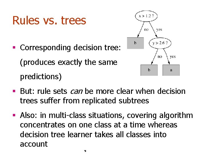
Rules vs. trees § Corresponding decision tree: (produces exactly the same predictions) § But: rule sets can be more clear when decision trees suffer from replicated subtrees § Also: in multi-class situations, covering algorithm concentrates on one class at a time whereas decision tree learner takes all classes into account 9

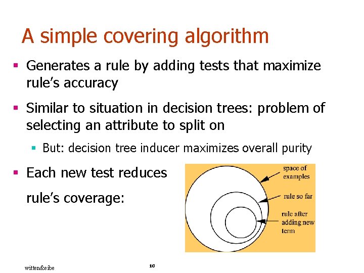
A simple covering algorithm § Generates a rule by adding tests that maximize rule’s accuracy § Similar to situation in decision trees: problem of selecting an attribute to split on § But: decision tree inducer maximizes overall purity § Each new test reduces rule’s coverage: witten&eibe 10

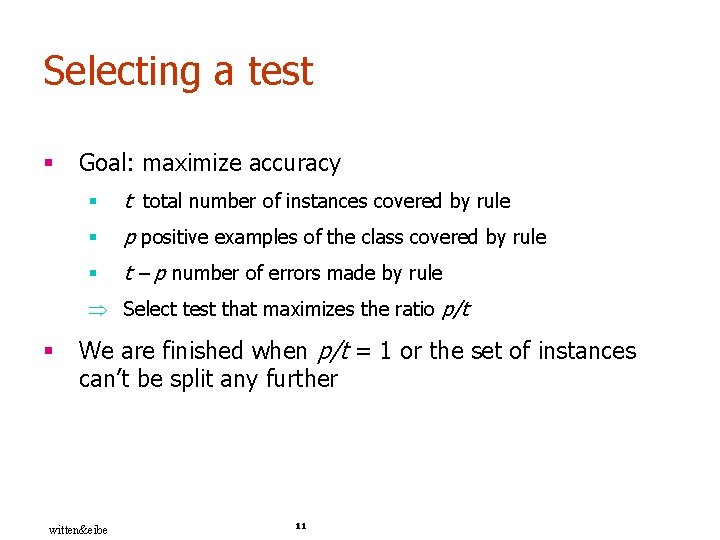
Selecting a test § Goal: maximize accuracy § t total number of instances covered by rule § p positive examples of the class covered by rule § t – p number of errors made by rule Select test that maximizes the ratio p/t § We are finished when p/t = 1 or the set of instances can’t be split any further witten&eibe 11

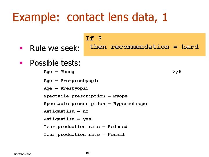
Example: contact lens data, 1 If ? § Rule we seek: then recommendation = hard § Possible tests: Age = Young 2/8 Age = Pre-presbyopic Age = Presbyopic Spectacle prescription = Myope Spectacle prescription = Hypermetrope Astigmatism = no Astigmatism = yes Tear production rate = Reduced Tear production rate = Normal witten&eibe 12

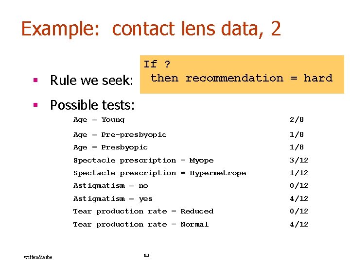
Example: contact lens data, 2 If ? § Rule we seek: then recommendation = hard § Possible tests: witten&eibe Age = Young 2/8 Age = Pre-presbyopic 1/8 Age = Presbyopic 1/8 Spectacle prescription = Myope 3/12 Spectacle prescription = Hypermetrope 1/12 Astigmatism = no 0/12 Astigmatism = yes 4/12 Tear production rate = Reduced 0/12 Tear production rate = Normal 4/12 13

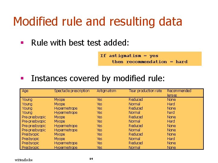
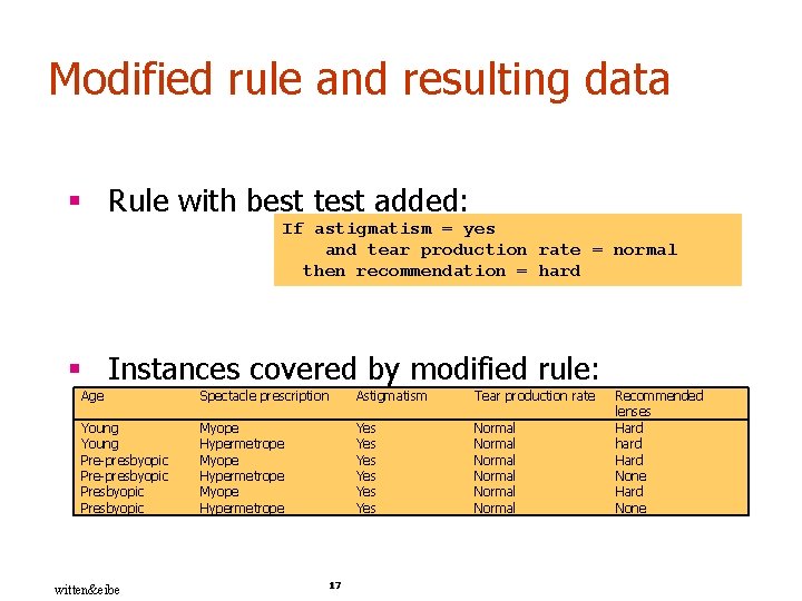
Modified rule and resulting data § Rule with best test added: If astigmatism = yes then recommendation = hard § Instances covered by modified rule: Age Spectacle prescription Astigmatism Tear production rate Young Pre-presbyopic Presbyopic Myope Hypermetrope Myope Hypermetrope Yes Yes Yes Reduced Normal Reduced Normal witten&eibe 14 Recommended lenses None Hard None hard None Hard None

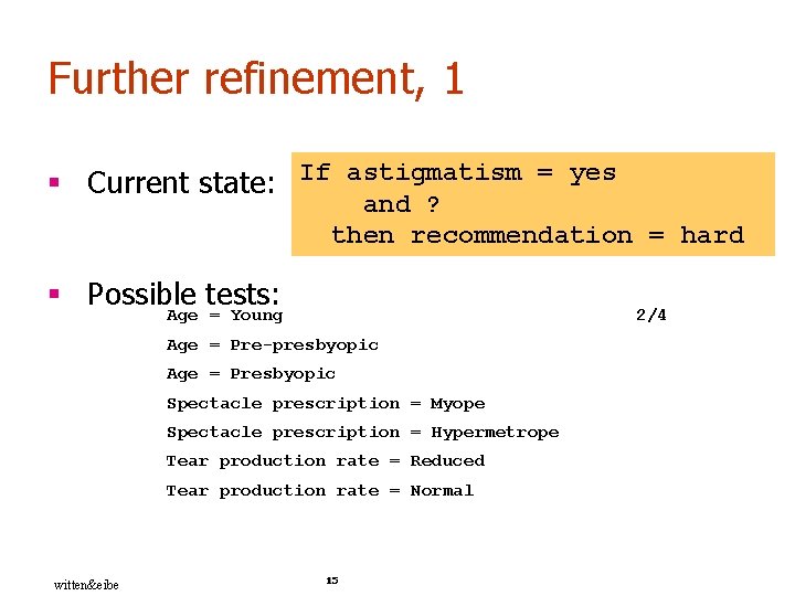
Further refinement, 1 § Current state: If astigmatism = yes and ? then recommendation = hard § Possible tests: Age = Young 2/4 Age = Pre-presbyopic Age = Presbyopic Spectacle prescription = Myope Spectacle prescription = Hypermetrope Tear production rate = Reduced Tear production rate = Normal witten&eibe 15

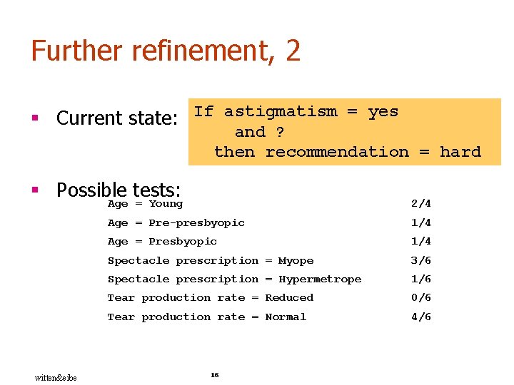
Further refinement, 2 § Current state: If astigmatism = yes and ? then recommendation = hard § Possible tests: Age = Young witten&eibe 2/4 Age = Pre-presbyopic 1/4 Age = Presbyopic 1/4 Spectacle prescription = Myope 3/6 Spectacle prescription = Hypermetrope 1/6 Tear production rate = Reduced 0/6 Tear production rate = Normal 4/6 16

Modified rule and resulting data § Rule with best test added: If astigmatism = yes and tear production rate = normal then recommendation = hard § Instances covered by modified rule: Age Spectacle prescription Astigmatism Tear production rate Young Pre-presbyopic Presbyopic Myope Hypermetrope Yes Yes Yes Normal Normal witten&eibe 17 Recommended lenses Hard hard Hard None

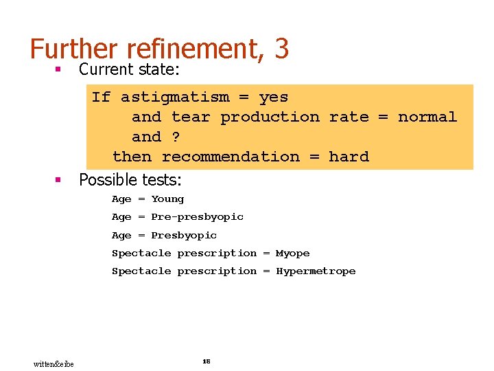
Further refinement, 3 § Current state: § If astigmatism = yes and tear production rate = normal and ? then recommendation = hard Possible tests: Age = Young Age = Pre-presbyopic Age = Presbyopic Spectacle prescription = Myope Spectacle prescription = Hypermetrope witten&eibe 18

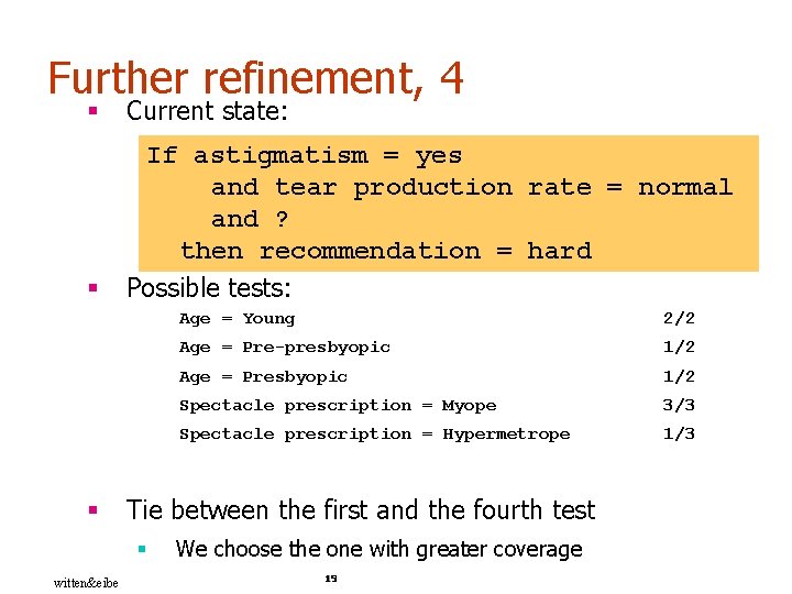
Further refinement, 4 § Current state: § If astigmatism = yes and tear production rate = normal and ? then recommendation = hard Possible tests: § 2/2 Age = Pre-presbyopic 1/2 Age = Presbyopic 1/2 Spectacle prescription = Myope 3/3 Spectacle prescription = Hypermetrope 1/3 Tie between the first and the fourth test § witten&eibe Age = Young We choose the one with greater coverage 19

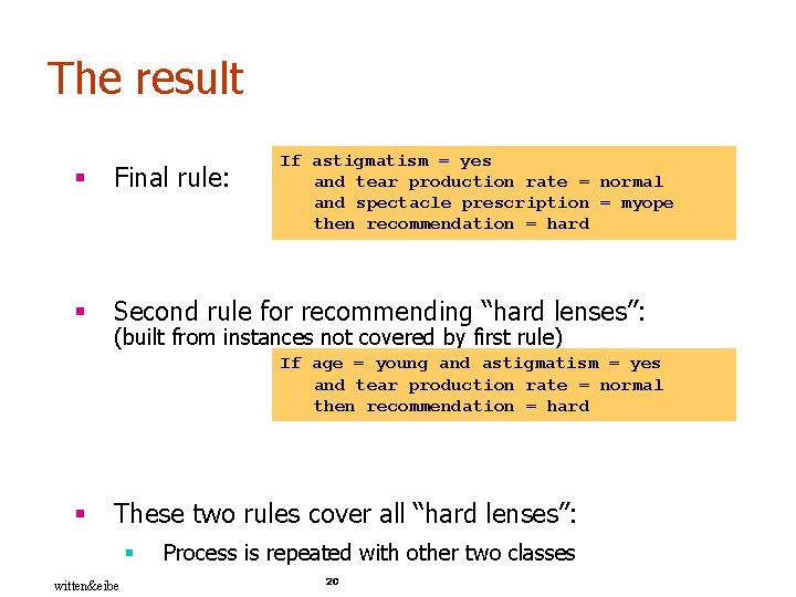
The result If astigmatism = yes and tear production rate = normal and spectacle prescription = myope then recommendation = hard § Final rule: § Second rule for recommending “hard lenses”: (built from instances not covered by first rule) If age = young and astigmatism = yes and tear production rate = normal then recommendation = hard § These two rules cover all “hard lenses”: § witten&eibe Process is repeated with other two classes 20

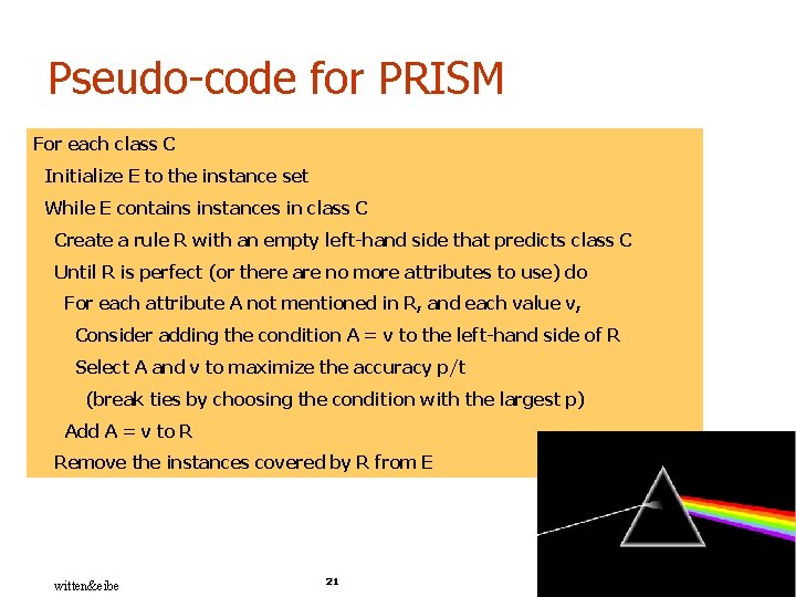
Pseudo-code for PRISM For each class C Initialize E to the instance set While E contains instances in class C Create a rule R with an empty left-hand side that predicts class C Until R is perfect (or there are no more attributes to use) do For each attribute A not mentioned in R, and each value v, Consider adding the condition A = v to the left-hand side of R Select A and v to maximize the accuracy p/t (break ties by choosing the condition with the largest p) Add A = v to R Remove the instances covered by R from E witten&eibe 21

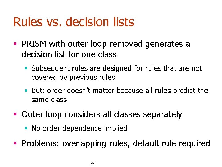
Rules vs. decision lists § PRISM with outer loop removed generates a decision list for one class § Subsequent rules are designed for rules that are not covered by previous rules § But: order doesn’t matter because all rules predict the same class § Outer loop considers all classes separately § No order dependence implied § Problems: overlapping rules, default rule required 22

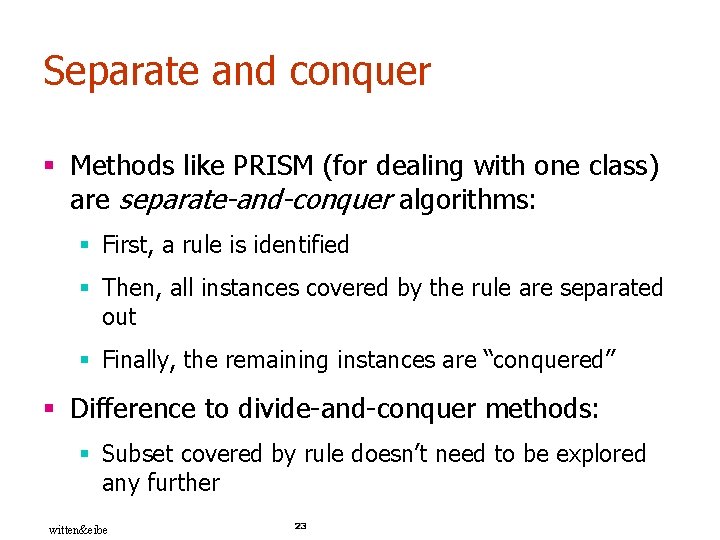
Separate and conquer § Methods like PRISM (for dealing with one class) are separate-and-conquer algorithms: § First, a rule is identified § Then, all instances covered by the rule are separated out § Finally, the remaining instances are “conquered” § Difference to divide-and-conquer methods: § Subset covered by rule doesn’t need to be explored any further witten&eibe 23

Outline § Rules § Linear Models (Regression) § Instance-based (Nearest-neighbor) 24

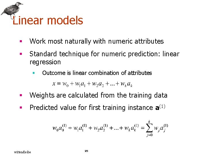
Linear models § Work most naturally with numeric attributes § Standard technique for numeric prediction: linear regression § Outcome is linear combination of attributes § Weights are calculated from the training data § Predicted value for first training instance a(1) witten&eibe 25

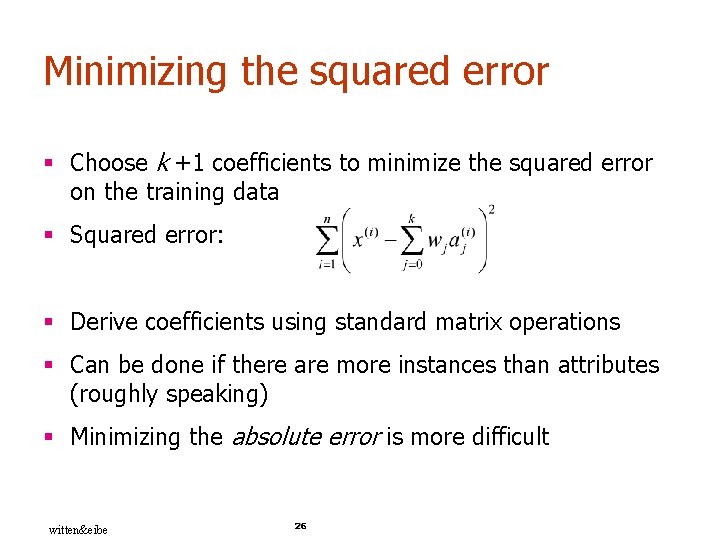
Minimizing the squared error § Choose k +1 coefficients to minimize the squared error on the training data § Squared error: § Derive coefficients using standard matrix operations § Can be done if there are more instances than attributes (roughly speaking) § Minimizing the absolute error is more difficult witten&eibe 26

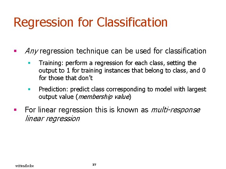
Regression for Classification § § Any regression technique can be used for classification § Training: perform a regression for each class, setting the output to 1 for training instances that belong to class, and 0 for those that don’t § Prediction: predict class corresponding to model with largest output value (membership value) For linear regression this is known as multi-response linear regression witten&eibe 27

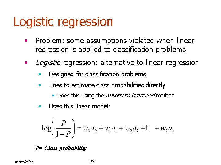
Logistic regression § Problem: some assumptions violated when linear regression is applied to classification problems § Logistic regression: alternative to linear regression § Designed for classification problems § Tries to estimate class probabilities directly § Does this using the maximum likelihood method § Uses this linear model: P= Class probability witten&eibe 30

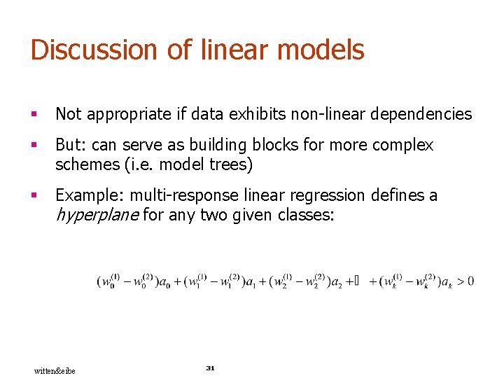
Discussion of linear models § Not appropriate if data exhibits non-linear dependencies § But: can serve as building blocks for more complex schemes (i. e. model trees) § Example: multi-response linear regression defines a hyperplane for any two given classes: witten&eibe 31

Comments on basic methods § Minsky and Papert (1969) showed that linear classifiers have limitations, e. g. can’t learn XOR § witten&eibe But: combinations of them can ( Neural Nets) 32

Outline § Rules § Linear Models (Regression) § Instance-based (Nearest-neighbor) 33

Instance-based representation § Simplest form of learning: rote learning § Training instances are searched for instance that most closely resembles new instance § The instances themselves represent the knowledge § Also called instance-based learning § Similarity function defines what’s “learned” § Instance-based learning is lazy learning § Methods: witten&eibe § nearest-neighbor § k-nearest-neighbor § … 34

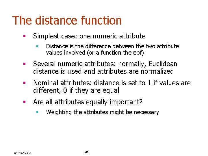
The distance function § Simplest case: one numeric attribute § Distance is the difference between the two attribute values involved (or a function thereof) § Several numeric attributes: normally, Euclidean distance is used and attributes are normalized § Nominal attributes: distance is set to 1 if values are different, 0 if they are equal § Are all attributes equally important? § witten&eibe Weighting the attributes might be necessary 35

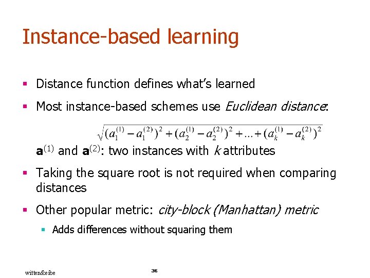
Instance-based learning § Distance function defines what’s learned § Most instance-based schemes use Euclidean distance: a(1) and a(2): two instances with k attributes § Taking the square root is not required when comparing distances § Other popular metric: city-block (Manhattan) metric § Adds differences without squaring them witten&eibe 36

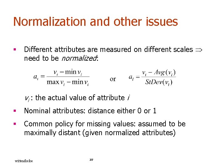
Normalization and other issues § Different attributes are measured on different scales need to be normalized: or vi : the actual value of attribute i § Nominal attributes: distance either 0 or 1 § Common policy for missing values: assumed to be maximally distant (given normalized attributes) witten&eibe 37

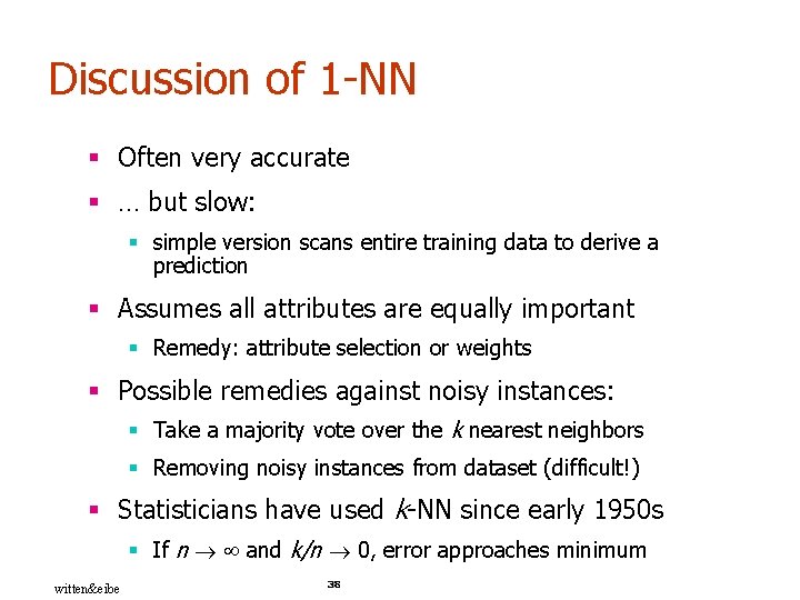
Discussion of 1 -NN § Often very accurate § … but slow: § simple version scans entire training data to derive a prediction § Assumes all attributes are equally important § Remedy: attribute selection or weights § Possible remedies against noisy instances: § Take a majority vote over the k nearest neighbors § Removing noisy instances from dataset (difficult!) § Statisticians have used k-NN since early 1950 s § If n and k/n 0, error approaches minimum witten&eibe 38

Summary § Simple methods frequently work well § robust against noise, errors § Advanced methods, if properly used, can improve on simple methods § No method is universally best 39

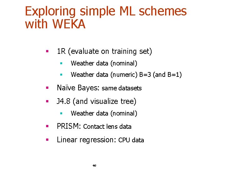
Exploring simple ML schemes with WEKA § 1 R (evaluate on training set) § Weather data (nominal) § Weather data (numeric) B=3 (and B=1) § Naïve Bayes: same datasets § J 4. 8 (and visualize tree) § Weather data (nominal) § PRISM: Contact lens data § Linear regression: CPU data 40