Classical Inference Two simple inference scenarios Question 1

"Classical" Inference

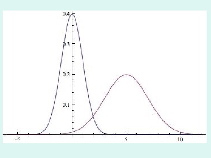
Two simple inference scenarios Question 1: Are we in world A or world B?

Possible worlds: World A World B X number added [-. 5, . 5] 38 38 [4, 6] 38 38 [-1, 1] 68 30 [3, 7] 68 30 [-1. 5, 1. 5] 87 19 [2, 8] 87 19 [-2, 2] 95 8 [1, 9] 95 8 [-2. 5, 2. 5] 99 4 [0, 10] 99 4 (- ∞, ∞) 100 1 100

Jerzy Neyman and Egon Pearson

D: Decision in favor of: T: The Truth of the matter: H 0: Null Hypothesis H 1: Alternative Hypothesis Correct acceptance Type I Error of H 0 pr(D=H 0| T=H 0) H 0: Null Hypothesis = (1 – ) Type II Error H 1: Alternative Hypothesis pr(D=H 0| T=H 1) = pr(D=H 1| T=H 0) = [aka size] Correct acceptance of H 1 pr(D=H 1| T=H 1) = (1 – ) [aka power]

Definition. A subset C of the sample space is a best critical region of size α for testing the hypothesis H 0 against the hypothesis H 1 if and for every subset A of the sample space, whenever: we also have:

Neyman-Pearson Theorem: Suppose that for some k > 0: 1. 2. 3. Then C is a best critical region of size α for the test of H 0 vs. H 1.

• When the null and alternative hypotheses are both Normal, the relation between the power of a statistical test (1 – ) and is given by the formula � is the cdf of N(0, 1), and q is the quantile determined by . • fixes the type I error probability, but increasing n reduces the type II error 9 probability

Question 2: Does the evidence suggest our world is not like World A?

World A X number added [-. 5, . 5] 38 38 [-1, 1] 68 30 [-1. 5, 1. 5] 87 19 [-2, 2] 95 8 [-2. 5, 2. 5] 99 4 (- ∞, ∞) 1 100

Sir Ronald Aymler Fisher

Fisherian theory Significance tests: their disjunctive logic, and p-values as evidence: ``[This very low p-value] is amply low enough to exclude at a high level of significance any theory involving a random distribution…. . The force with which such a conclusion is supported is logically that of the simple disjunction: Either an exceptionally rare chance has occurred, or theory of random distribution is not true. '' (Fisher 1959, 39)

Fisherian theory ``The meaning of `H' is rejected at level α' is `Either an event of probability α has occurred, or H is false', and our disposition to disbelieve H arises from our disposition to disbelieve in events of small probability. '' (Barnard 1967, 32)

• • Fisherian theory: Distinctive features Notice that the actual data x is used to define the event whose significance is evaluated. • Also based on H 0 and H 1 Can only reject H 0, evidence cannot allow one to accept H 0. • Many other theories besides H 0 could also explain the data.

• Common philosophical simplification: • Hypothesis space given qualitatively; • H 0 vs. –H 0, • Murderer was Professor Plum, Colonel Mustard, Miss Scarlett, or Mrs. Peacock • More typical situation: • Very strong structural assumptions • Hypothesis space given by unknown numeric `parameters' • Test uses: • a transformation of the raw data, • a probability distribution for this transformation (≠ the original distribution of interest)

Three Commonly Used Facts • Assume is a collection of independent and identically distributed (i. i. d. ) random variables. • Assume also that the Xis share a mean of μ and a standard deviation of σ.

Three Commonly Used Facts For the mean estimator 1. 2. :

Three Commonly Used Facts The Central Limit Theorem. If {X 1, …, Xn} are i. i. d. random variables from a distribution with mean and variance 2, then: 3. Equivalently:

Examples • Data: January 2012 CPS • Sample: Ph. D’s, working full time, age 2834 • H 0: mean income is 75 k

21996. 00 89999. 52 119999. 9 40999. 92 67600. 00 68640. 00 96999. 76 77296. 96 65000. 00 71999. 72 100100. 0 45999. 72 149999. 7 19968. 00 10140. 00 37999. 52 74999. 60 69992. 00 31740. 80 65000. 00 57512. 00 87984. 00 35999. 60 38939. 68 99999. 64 74999. 60 149999. 7 47996. 00 62920. 00 54999. 88 104000. 0

Hyp. H 0 Value -1. 024022 Probability 0. 3138

Comments • The background conditions (e. g. , the i. i. d. condition behind the sample) are a clear example of `Quine-Duhem’ conditions. • When background conditions are met, ``large samples’’ don’t make inferences ``more certain’’ • Multiple tests • Monitoring or ``peeking'‘ at data, etc.

Point estimates and Confidence Intervals

• Many desiderata of an estimator: • • Consistent Maximum Likelihood Unbiased Sufficient Minimum variance Minimum MSE (mean squared error) (most) efficient

• By CLT: approximately: • Thus: • By algebra: • So:

Interpreting confidence intervals • The only probabilistic component that determines what occurs is. • Everything else are constants. • Simulations, examples • Question: Why ``center’’ the interval?

Confidence Intervals • $68, 898. 16 ± $12, 152. 85 • ``C. I. = mean ± m. o. e’’ • = ($56, 745. 32 , $81, 051. 01)

Using similar logic, but different computing formulae, one can extend these methods to address further questions e. g. , for standard deviations, equality of means across groups, etc.

Equality of Means: BAs Sex 1 2 All Count 223 209 432 Value 4. 424943 Mean 63619. 54 51395. 43 57705. 56 Std. Dev. 31370. 01 25530. 66 29306. 13 Probability 0. 0000

Equality of Means: Ph. Ds Sex Count Mean 1 21 2 11 All 32 Value -0. 560745 Std. Dev. 66452. 71 73566. 76 36139. 78 29555. 10 68898. 16 33707. 49 Probability 0. 5791