Classical Decomposition Boise State University By Kurt Folke
Classical Decomposition Boise State University By: Kurt Folke Spring 2003
Overview: • Time series models & classical decomposition • Brainstorming exercise • Classical decomposition explained • Classical decomposition illustration • Exercise • Summary • Bibliography & readings list • Appendix A: exercise templates
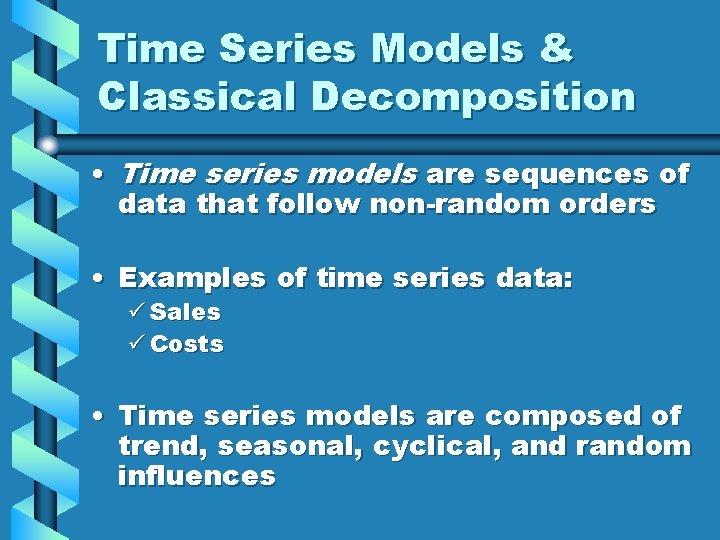
Time Series Models & Classical Decomposition • Time series models are sequences of data that follow non-random orders • Examples of time series data: ü Sales ü Costs • Time series models are composed of trend, seasonal, cyclical, and random influences
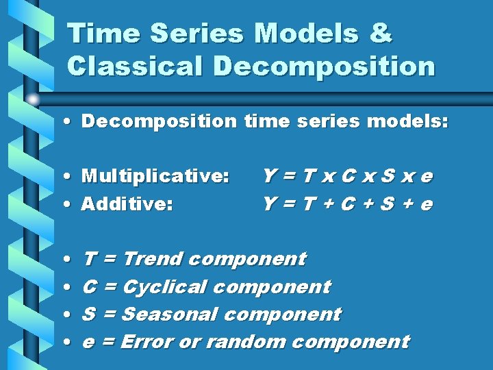
Time Series Models & Classical Decomposition • Decomposition time series models: • Multiplicative: • Additive: • • Y=Tx. Cx. Sxe Y=T+C+S+e T = Trend component C = Cyclical component S = Seasonal component e = Error or random component
Time Series Models & Classical Decomposition • Classical decomposition is used to isolate trend, seasonal, and other variability components from a time series model • Benefits: ü Shows fluctuations in trend ü Provides insight to underlying factors affecting the time series

Brainstorming Exercise • Identify how this tool can be used in your organization…
Classical Decomposition Explained Basic Steps: 1. Determine seasonal indexes using the ratio to moving average method 2. Deseasonalize the data 3. Develop the trend-cyclical regression equation using deseasonalized data 4. Multiply the forecasted trend values by their seasonal indexes to create a more accurate forecast
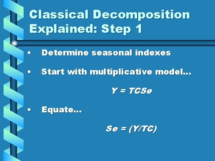
Classical Decomposition Explained: Step 1 • Determine seasonal indexes • Start with multiplicative model… Y = TCSe • Equate… Se = (Y/TC)
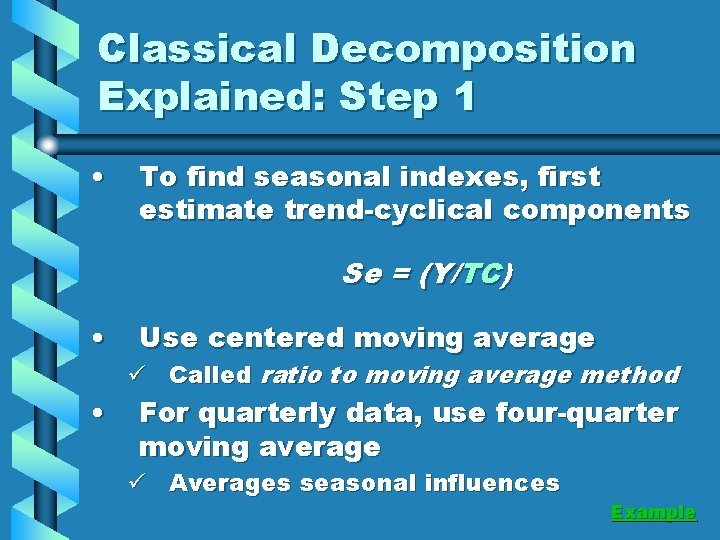
Classical Decomposition Explained: Step 1 • To find seasonal indexes, first estimate trend-cyclical components Se = (Y/TC) • • Use centered moving average ü Called ratio to moving average method For quarterly data, use four-quarter moving average ü Averages seasonal influences Example
Classical Decomposition Explained: Step 1 • Four-quarter moving average will position average at… ü end of second period and ü beginning of third period • Use centered moving average to position data in middle of the period Example
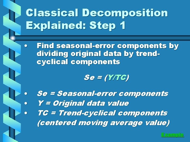
Classical Decomposition Explained: Step 1 • Find seasonal-error components by dividing original data by trendcyclical components Se = (Y/TC) • • • Se = Seasonal-error components Y = Original data value TC = Trend-cyclical components (centered moving average value) Example
Classical Decomposition Explained: Step 1 • Unadjusted seasonal indexes (USI) are found by averaging seasonalerror components by period Example • Develop adjusting factor (AF) so USIs are adjusted so their sum equals the number of quarters (4) ü Reduces error Example
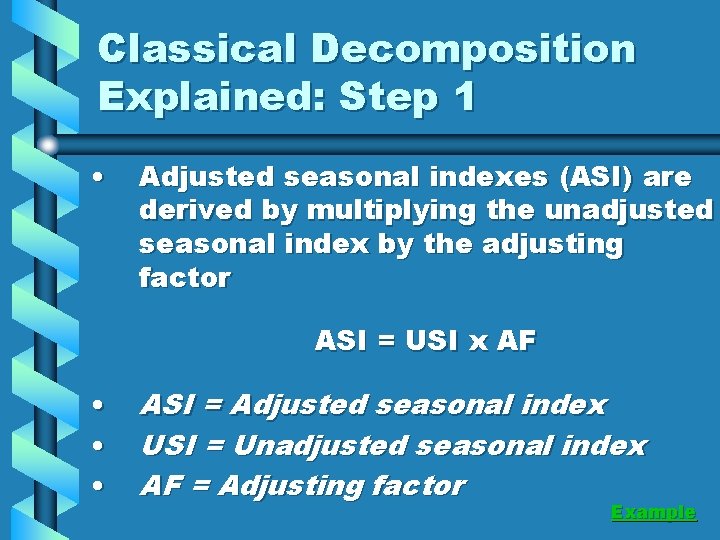
Classical Decomposition Explained: Step 1 • Adjusted seasonal indexes (ASI) are derived by multiplying the unadjusted seasonal index by the adjusting factor ASI = USI x AF • • • ASI = Adjusted seasonal index USI = Unadjusted seasonal index AF = Adjusting factor Example
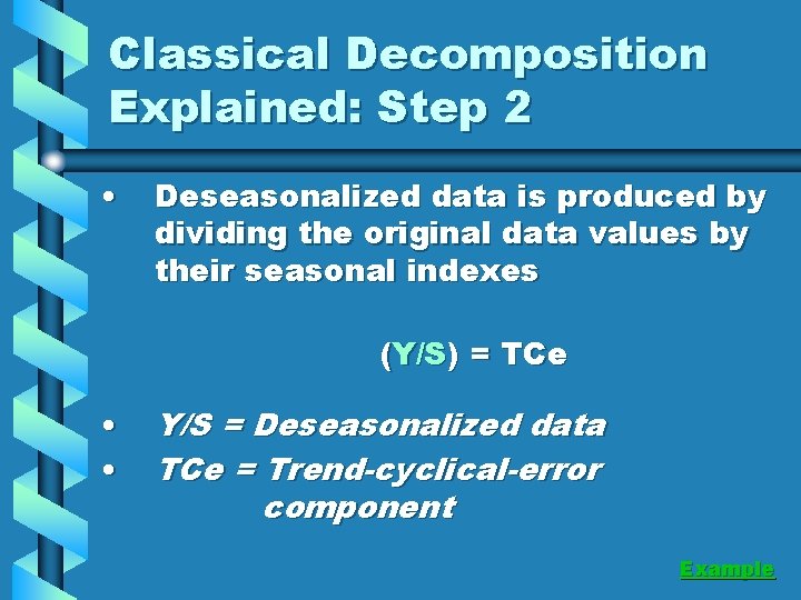
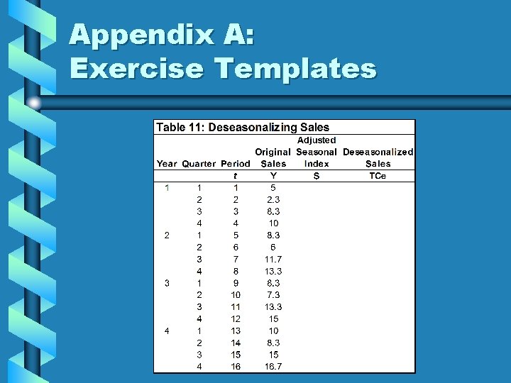
Classical Decomposition Explained: Step 2 • Deseasonalized data is produced by dividing the original data values by their seasonal indexes (Y/S) = TCe • • Y/S = Deseasonalized data TCe = Trend-cyclical-error component Example

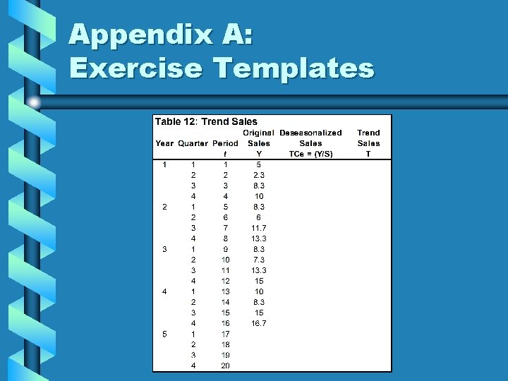
Classical Decomposition Explained: Step 3 • Develop the trend-cyclical regression equation using deseasonalized data Tt = a + bt • • • Tt = Trend value at period t a = Intercept value b = Slope of trend line Example
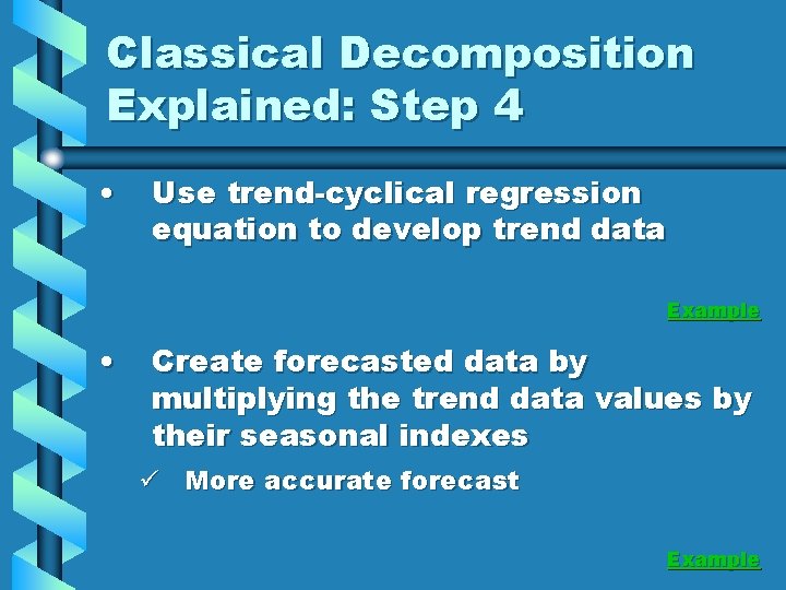
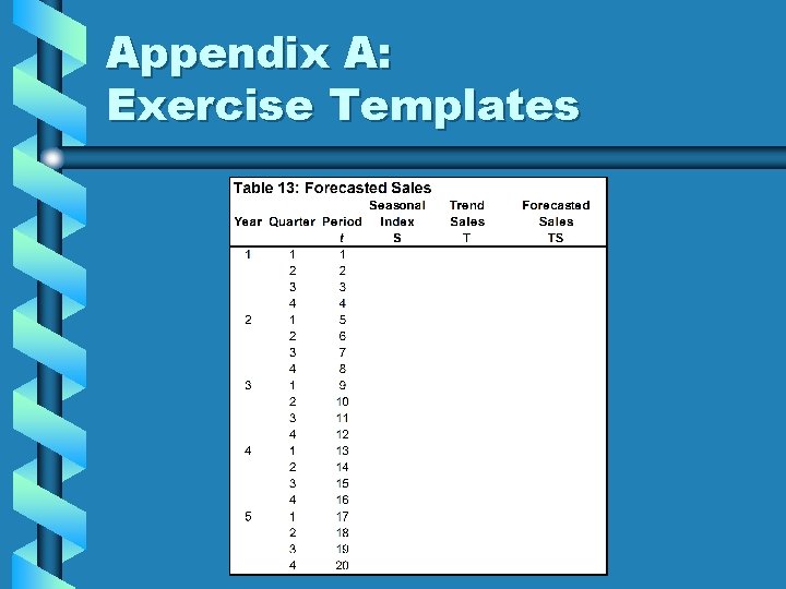
Classical Decomposition Explained: Step 4 • Use trend-cyclical regression equation to develop trend data Example • Create forecasted data by multiplying the trend data values by their seasonal indexes ü More accurate forecast Example
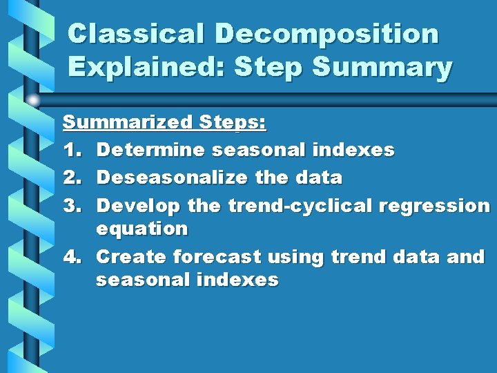
Classical Decomposition Explained: Step Summary Summarized Steps: 1. Determine seasonal indexes 2. Deseasonalize the data 3. Develop the trend-cyclical regression equation 4. Create forecast using trend data and seasonal indexes
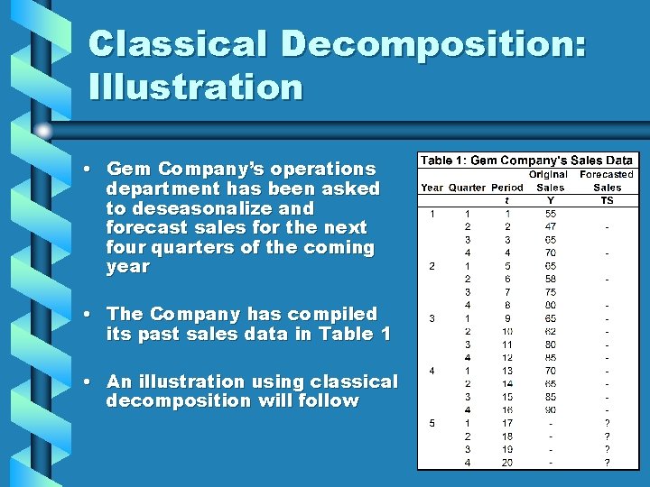
Classical Decomposition: Illustration • Gem Company’s operations department has been asked to deseasonalize and forecast sales for the next four quarters of the coming year • The Company has compiled its past sales data in Table 1 • An illustration using classical decomposition will follow
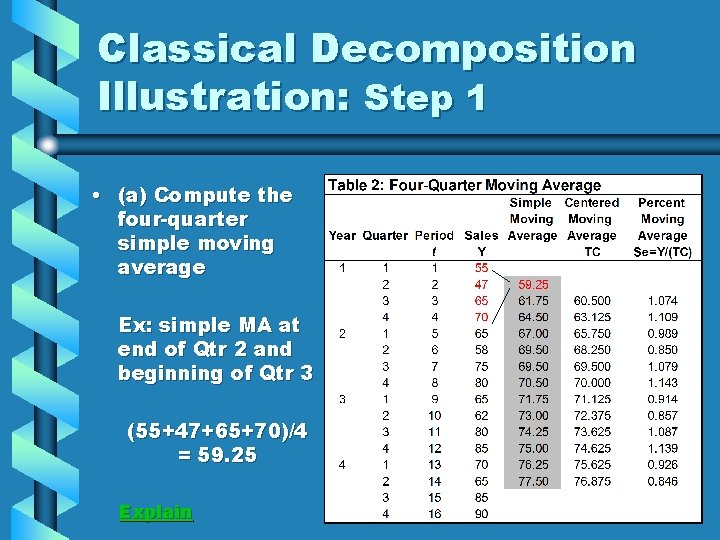
Classical Decomposition Illustration: Step 1 • (a) Compute the four-quarter simple moving average Ex: simple MA at end of Qtr 2 and beginning of Qtr 3 (55+47+65+70)/4 = 59. 25 Explain
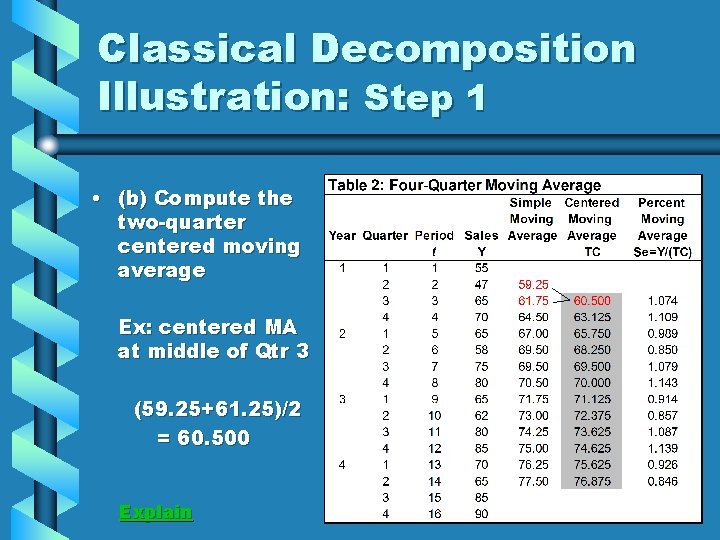
Classical Decomposition Illustration: Step 1 • (b) Compute the two-quarter centered moving average Ex: centered MA at middle of Qtr 3 (59. 25+61. 25)/2 = 60. 500 Explain
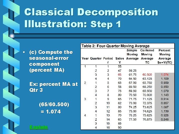
Classical Decomposition Illustration: Step 1 • (c) Compute the seasonal-error component (percent MA) Ex: percent MA at Qtr 3 (65/60. 500) = 1. 074 Explain
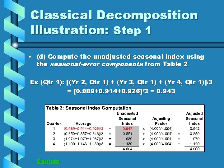
Classical Decomposition Illustration: Step 1 • (d) Compute the unadjusted seasonal index using the seasonal-error components from Table 2 Ex (Qtr 1): [(Yr 2, Qtr 1) + (Yr 3, Qtr 1) + (Yr 4, Qtr 1)]/3 = [0. 989+0. 914+0. 926]/3 = 0. 943 Explain
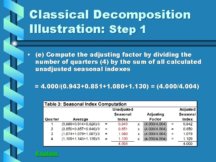
Classical Decomposition Illustration: Step 1 • (e) Compute the adjusting factor by dividing the number of quarters (4) by the sum of all calculated unadjusted seasonal indexes = 4. 000/(0. 943+0. 851+1. 080+1. 130) = (4. 000/4. 004) Explain
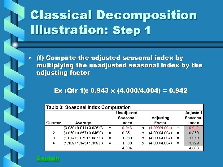
Classical Decomposition Illustration: Step 1 • (f) Compute the adjusted seasonal index by multiplying the unadjusted seasonal index by the adjusting factor Ex (Qtr 1): 0. 943 x (4. 000/4. 004) = 0. 942 Explain
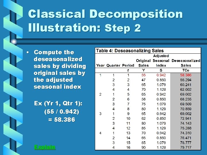
Classical Decomposition Illustration: Step 2 • Compute the deseasonalized sales by dividing original sales by the adjusted seasonal index Ex (Yr 1, Qtr 1): (55 / 0. 942) = 58. 386 Explain
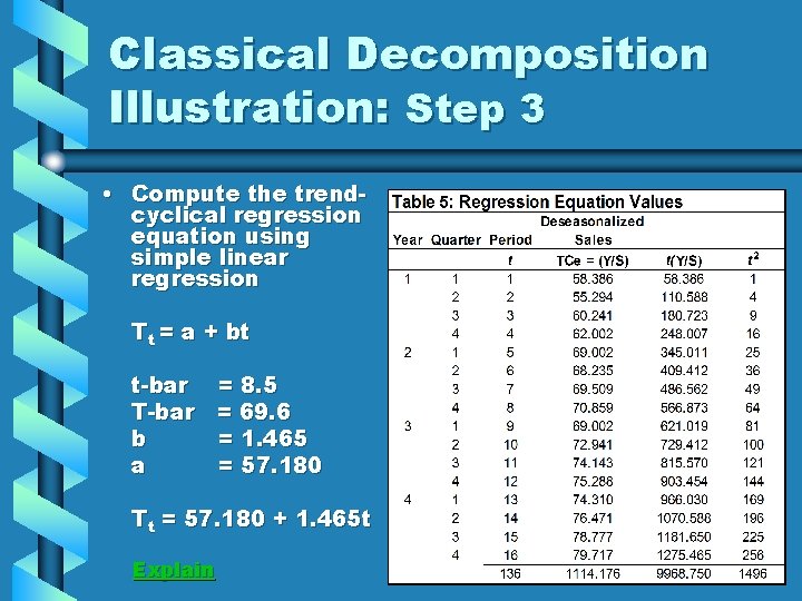
Classical Decomposition Illustration: Step 3 • Compute the trendcyclical regression equation using simple linear regression Tt = a + bt t-bar = 8. 5 T-bar = 69. 6 b = 1. 465 a = 57. 180 Tt = 57. 180 + 1. 465 t Explain
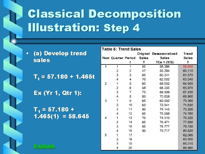
Classical Decomposition Illustration: Step 4 • (a) Develop trend sales Tt = 57. 180 + 1. 465 t Ex (Yr 1, Qtr 1): T 1 = 57. 180 + 1. 465(1) = 58. 645 Explain
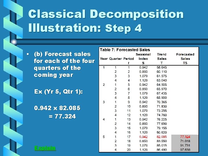
Classical Decomposition Illustration: Step 4 • (b) Forecast sales for each of the four quarters of the coming year Ex (Yr 5, Qtr 1): 0. 942 x 82. 085 = 77. 324 Explain
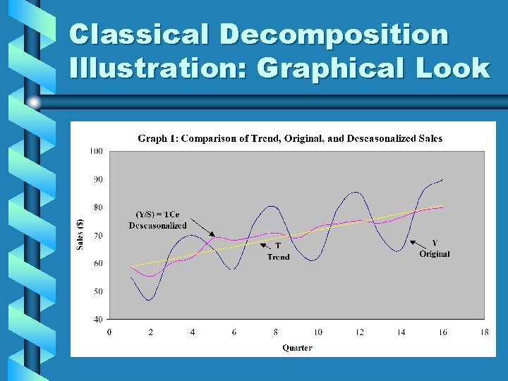
Classical Decomposition Illustration: Graphical Look
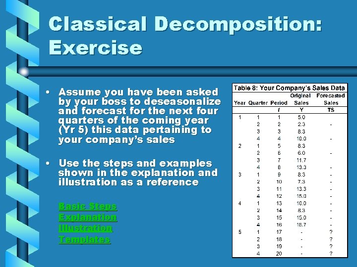
Classical Decomposition: Exercise • Assume you have been asked by your boss to deseasonalize and forecast for the next four quarters of the coming year (Yr 5) this data pertaining to your company’s sales • Use the steps and examples shown in the explanation and illustration as a reference Basic Steps Explanation Illustration Templates
Summary • Time series models are sequences of data that follow non-arbitrary orders • Classical decomposition isolates the components of a time series model • Benefits: üInsight to fluctuations in trend üDecomposes the underlying factors affecting the time series
Bibliography & Readings List De. Lurgio, Stephen, and Bhame, Carl. Forecasting Systems for Operations Management. Homewood: Business One Irwin, 1991. Shim, Jae K. Strategic Business Forecasting. New York: St Lucie, 2000. Stat. Soft Inc. (2003). Time Series Analysis. Retrieved April 21, 2003, from http: //www. statsoft. com/textbook/sttimser. html
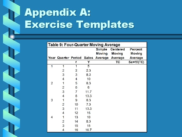
Appendix A: Exercise Templates
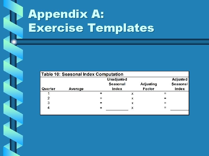
Appendix A: Exercise Templates
Appendix A: Exercise Templates
Appendix A: Exercise Templates
Appendix A: Exercise Templates
- Slides: 37