Classic model Wilson 1934 in this classic paper

Classic model • Wilson (1934), in this classic paper, he breaks the inventory control problem into two distinct parts: • 1. Determining the order quantity, which is the amount of inventory that will be purchased or produced with each replenishment. • 2. Determining the reorder point, or the inventory level at which a replenishment (purchase or production) will be triggered.

First part: replenishment • In this section, we address this two‑part problem in three stages (two classes): First, we consider the situation where we are only interested in a single replenishment, so that the only issue is to determine the appropriate order quantity in the face of uncertain demand. This has traditionally been called the newsboy model because it could apply to a person who purchases newspapers at the beginning of the day, sells a random amount, and then must discard any leftovers.

Second part: reorder point • Second, we consider the situation where inventory is replenished one unit at a time as random demands occur, so that the only issue is to determine the reorder point. The target inventory level we set for the system is known as a base stock level, and hence the resulting model is termed the base stock model.

Third part: (Q, r) model • Third, we consider the situation where inventory is monitored continuously and demands occur randomly, possibly in batches. When the inventory level reaches (or goes below) r, an order of size Q is placed. After a lead time of l, during which a stockout might occur, the order is received. The problem is to de termine appropriate values of Q and r. The model we use to address this problem is known as the (Q, r) model

The Newboys model • Consider the situation a manufacturer of Christmas lights faces each year. Demand is somewhat unpredictable and occurs in such a short burst just prior to Christmas that if the inventory is not on the shelves, the demand will be lost. Therefore, the decision of how many sets of lights to produce must be made prior to the holiday season. Additionally, the cost of collecting unsold inventory and holding it until next year is too high to make year‑to‑year storage an attractive option. Instead, any unsold sets of lights are sold after Christmas at a steep discount.

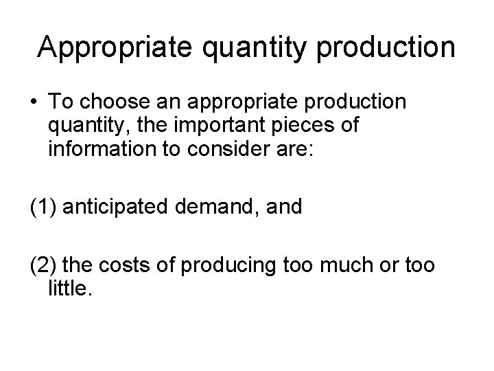
Appropriate quantity production • To choose an appropriate production quantity, the important pieces of information to consider are: (1) anticipated demand, and (2) the costs of producing too much or too little.

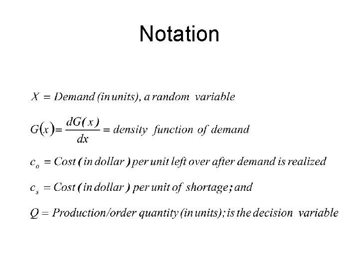
Notation

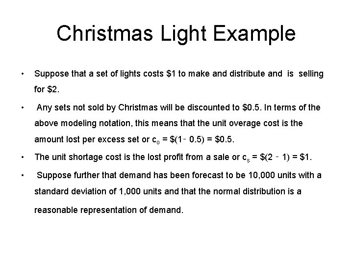
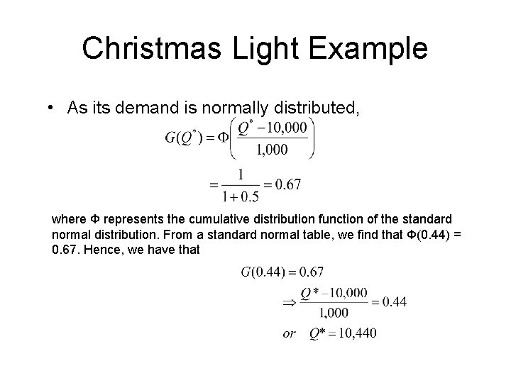
Christmas Light Example • Suppose that a set of lights costs $1 to make and distribute and is selling for $2. • Any sets not sold by Christmas will be discounted to $0. 5. In terms of the above modeling notation, this means that the unit overage cost is the amount lost per excess set or co = $(1‑ 0. 5) = $0. 5. • The unit shortage cost is the lost profit from a sale or cs = $(2 ‑ 1) = $1. • Suppose further that demand has been forecast to be 10, 000 units with a standard deviation of 1, 000 units and that the normal distribution is a reasonable representation of demand.

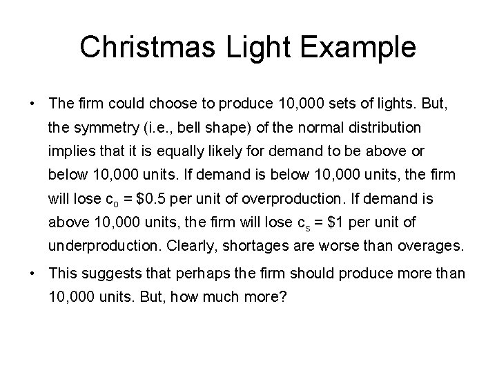
Christmas Light Example • The firm could choose to produce 10, 000 sets of lights. But, the symmetry (i. e. , bell shape) of the normal distribution implies that it is equally likely for demand to be above or below 10, 000 units. If demand is below 10, 000 units, the firm will lose co = $0. 5 per unit of overproduction. If demand is above 10, 000 units, the firm will lose cs = $1 per unit of underproduction. Clearly, shortages are worse than overages. • This suggests that perhaps the firm should produce more than 10, 000 units. But, how much more?

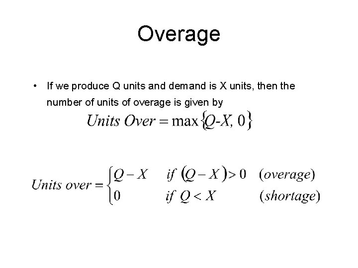
Overage • If we produce Q units and demand is X units, then the number of units of overage is given by

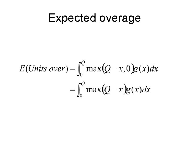
Expected overage

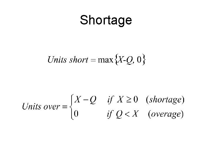
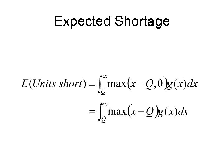
Shortage

Expected Shortage

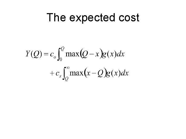
The expected cost

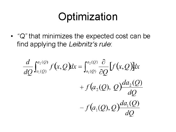
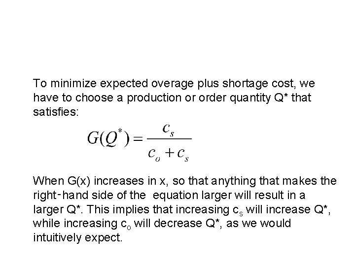
Optimization • “Q” that minimizes the expected cost can be find applying the Leibnitz's rule:

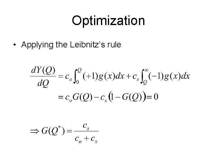
Optimization • Applying the Leibnitz’s rule

To minimize expected overage plus shortage cost, we have to choose a production or order quantity Q* that satisfies: When G(x) increases in x, so that anything that makes the right‑hand side of the equation larger will result in a larger Q*. This implies that increasing cs will increase Q*, while increasing co will decrease Q*, as we would intuitively expect.

Christmas Light Example • As its demand is normally distributed, where Ф represents the cumulative distribution function of the standard normal distribution. From a standard normal table, we find that Ф(0. 44) = 0. 67. Hence, we have that