Class Notes 1 Introduction MAE 82 Engineering Mathematics

Class Notes 1: Introduction MAE 82 – Engineering Mathematics

CHANGE

Rate of Change

Basic Mathematical Models • Many of the principles, or laws, underlying the behavior of the natural world are statements or relations involving rates at which things happen. • Principles / Laws – Relations -> Equations – Rates -> Derivative • A differential equation that describes a physical process is often called a mathematical model.

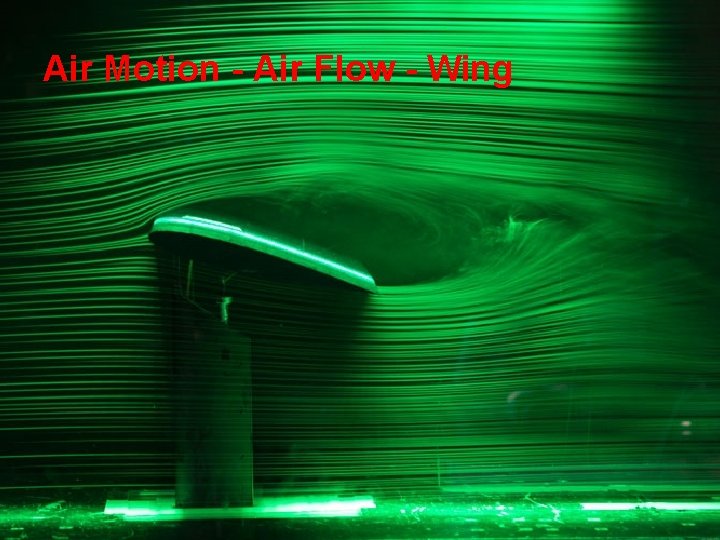
Air Motion - Air Flow - Wing

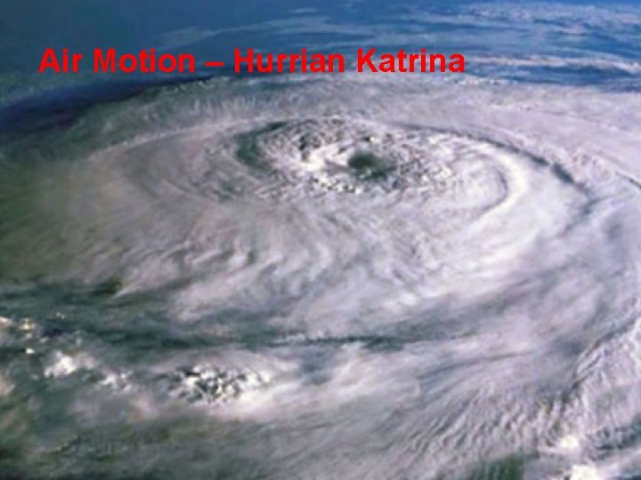
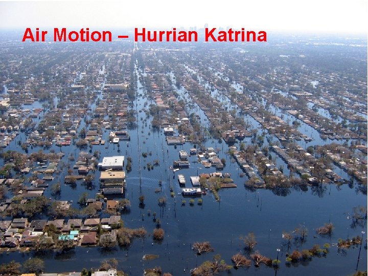
Air Motion – Hurrian Katrina

Air Motion – Hurrian Katrina

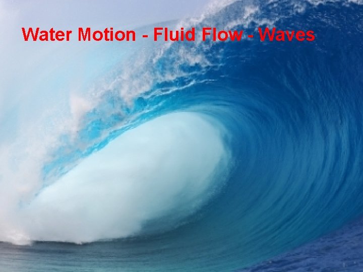
Water Motion - Fluid Flow - Waves

Water Motion - Fluid Flow - Waves 2004 Indian Ocean earthquake and tsunami

Solid Flow

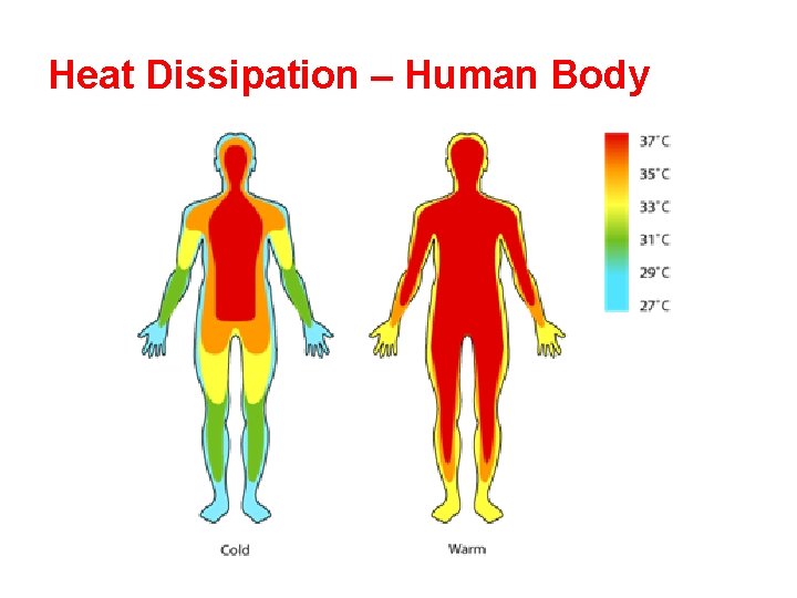
Heat Dissipation – Human Body

Population Dynamics

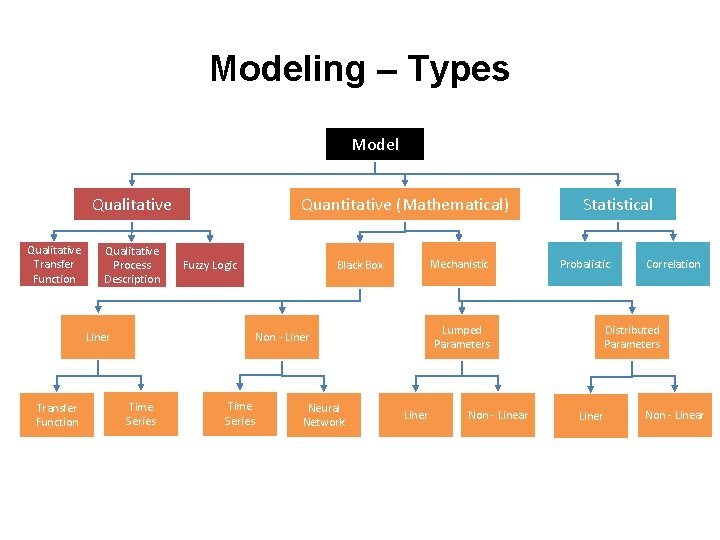
Modeling – Types Model Qualitative Transfer Function Qualitative Process Description Quantitative (Mathematical) Fuzzy Logic Liner Transfer Function Mechanistic Black Box Time Series Neural Network Probalistic Lumped Parameters Non - Liner Time Series Statistical Liner Non - Linear Correlation Distributed Parameters Liner Non - Linear

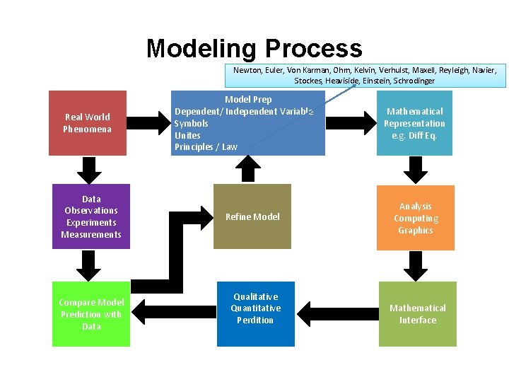
Modeling Process Newton, Euler, Von Karman, Ohm, Kelvin, Verhulst, Maxell, Reyleigh, Navier, Stockes, Heaviside, Einstein, Schrodinger Real World Phenomena Data Observations Experiments Measurements Compare Model Prediction with Data Model Prep Dependent/ Independent Variable Symbols Unites Principles / Law Refine Model Qualitative Quantitative Perdition Mathematical Representation e. g. Diff Eq. Analysis Computing Graphics Mathematical Interface

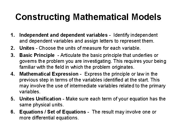
Constructing Mathematical Models 1. Independent and dependent variables - Identify independent and dependent variables and assign letters to represent them. 2. Unites - Choose the units of measure for each variable. 3. Basic Principle - Articulate the basic principle that underlies or governs the problem you are investigating. This requires your being familiar with the field in which the problem originates. 4. Mathematical Expression - Express the principle or law in the previous step in terms of the variables identified at the start. This may involve the use of intermediate variables related to the primary variables. 5. Unites Unification - Make sure each term of your equation has the same physical units. 6. Equations / Set of Equations - The result may involve one or more differential equations.

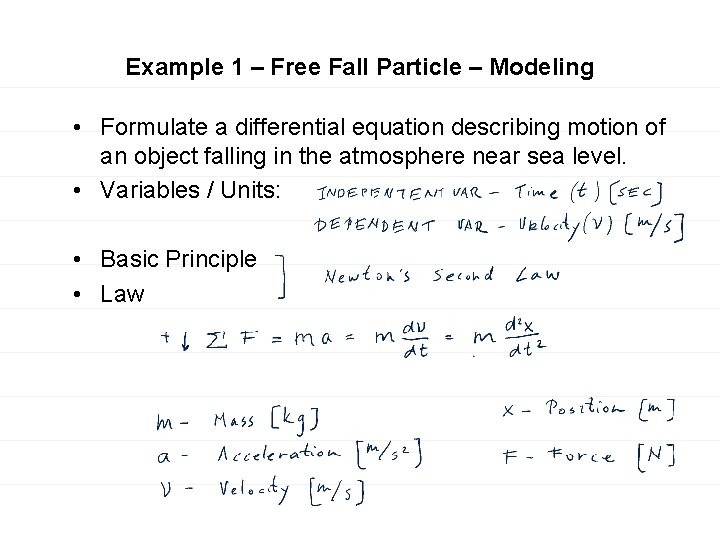
Example 1 – Free Fall Particle – Modeling • Formulate a differential equation describing motion of an object falling in the atmosphere near sea level. • Variables / Units: • Basic Principle • Law

Example 1 – Free Fall Particle – Modeling

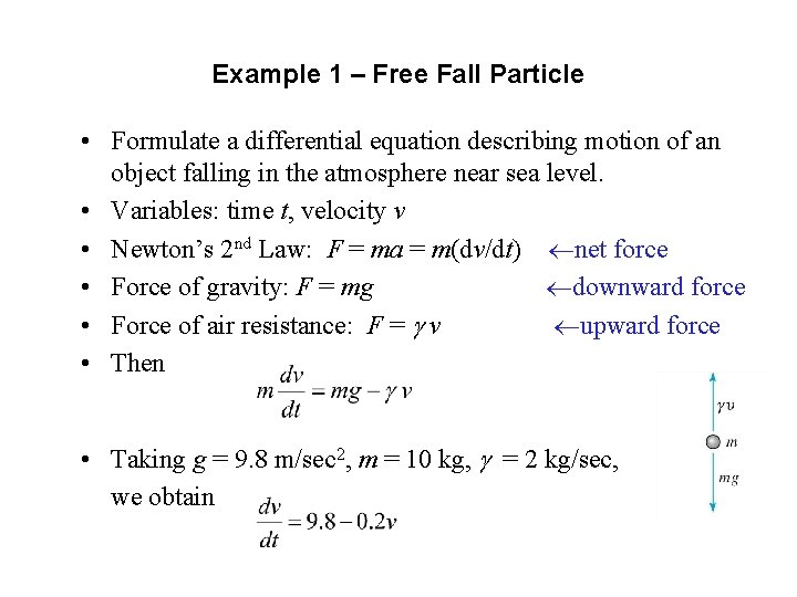
Example 1 – Free Fall Particle • Formulate a differential equation describing motion of an object falling in the atmosphere near sea level. • Variables: time t, velocity v • Newton’s 2 nd Law: F = ma = m(dv/dt) net force • Force of gravity: F = mg downward force • Force of air resistance: F = v upward force • Then • Taking g = 9. 8 m/sec 2, m = 10 kg, = 2 kg/sec, we obtain

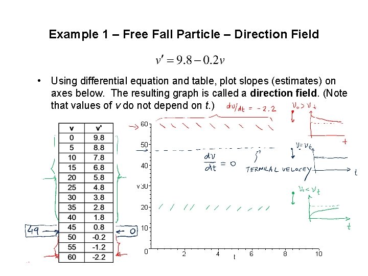
Example 1 – Free Fall Particle – Direction Field • Using differential equation and table, plot slopes (estimates) on axes below. The resulting graph is called a direction field. (Note that values of v do not depend on t. )

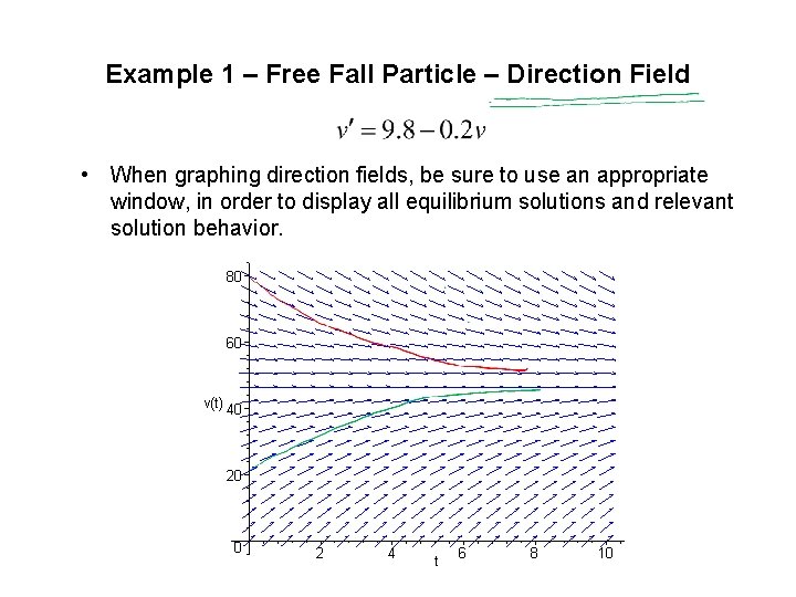
Example 1 – Free Fall Particle – Direction Field • When graphing direction fields, be sure to use an appropriate window, in order to display all equilibrium solutions and relevant solution behavior.

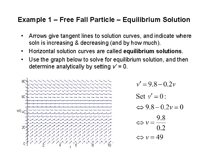
Example 1 – Free Fall Particle – Equilibrium Solution • Arrows give tangent lines to solution curves, and indicate where soln is increasing & decreasing (and by how much). • Horizontal solution curves are called equilibrium solutions. • Use the graph below to solve for equilibrium solution, and then determine analytically by setting v' = 0.

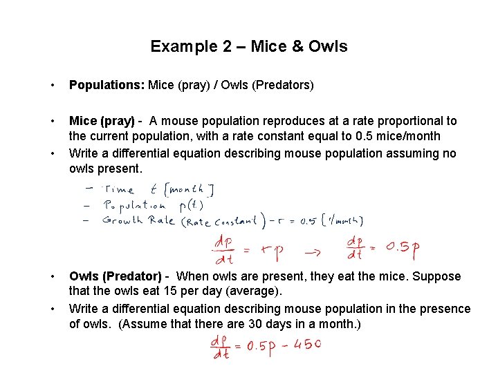
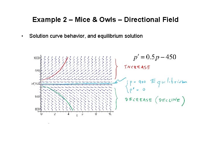
Example 2 – Mice & Owls • Populations: Mice (pray) / Owls (Predators) • Mice (pray) - A mouse population reproduces at a rate proportional to the current population, with a rate constant equal to 0. 5 mice/month Write a differential equation describing mouse population assuming no owls present. • • • Owls (Predator) - When owls are present, they eat the mice. Suppose that the owls eat 15 per day (average). Write a differential equation describing mouse population in the presence of owls. (Assume that there are 30 days in a month. )

Example 2 – Mice & Owls – Directional Field • Solution curve behavior, and equilibrium solution

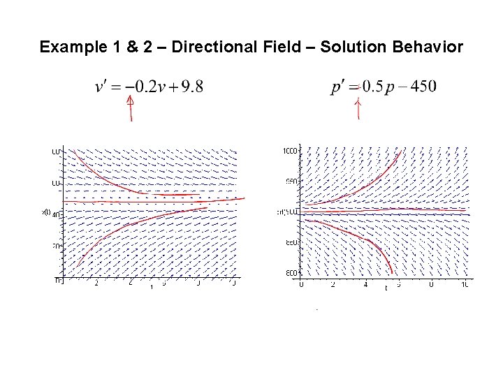
Example 1 & 2 – Directional Field – Solution Behavior

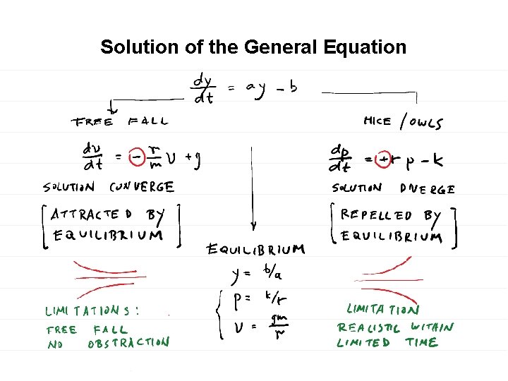
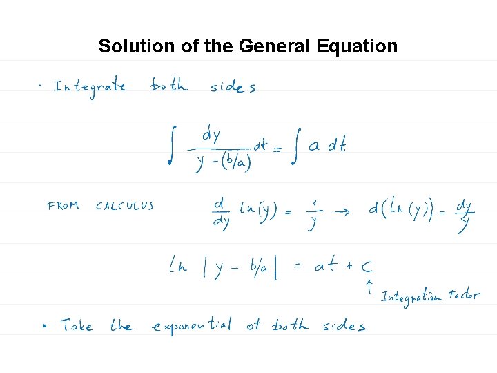
Solution of the General Equation

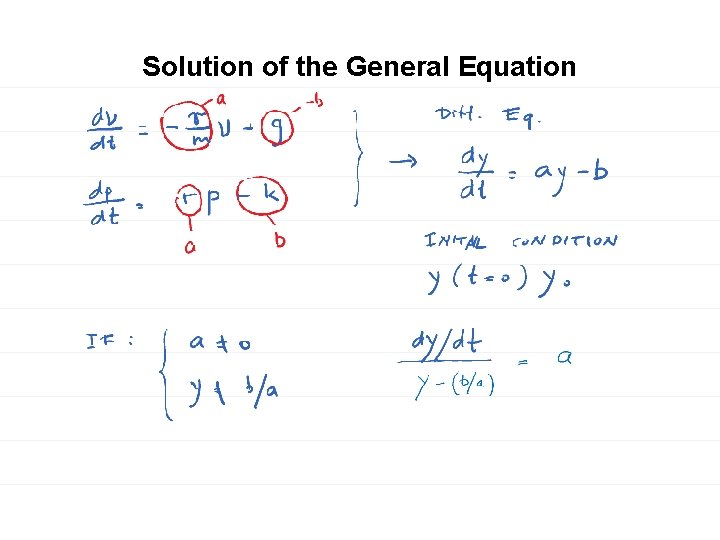
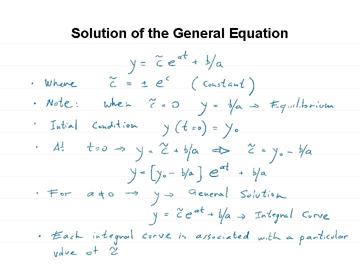
Solution of the General Equation

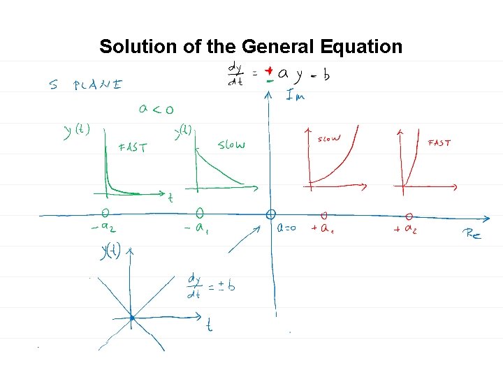
Solution of the General Equation

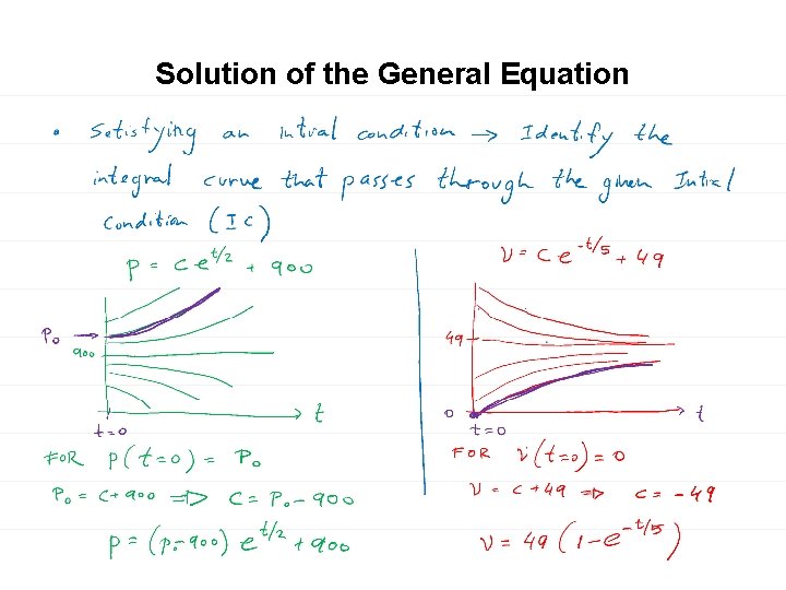
Solution of the General Equation

Solution of the General Equation

Solution of the General Equation

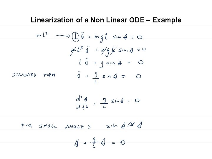
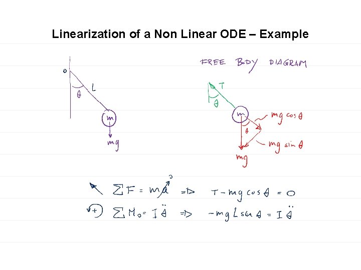
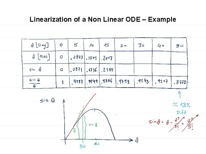
Linearization of a Non Linear ODE – Example

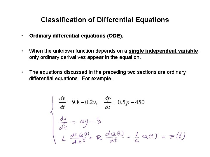
Classification of Differential Equations • Ordinary differential equations (ODE). • When the unknown function depends on a single independent variable, only ordinary derivatives appear in the equation. • The equations discussed in the preceding two sections are ordinary differential equations. For example,

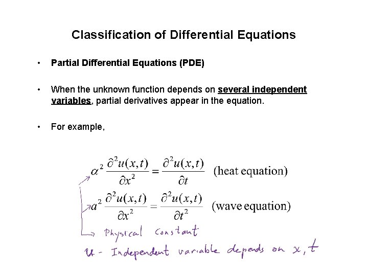
Classification of Differential Equations • Partial Differential Equations (PDE) • When the unknown function depends on several independent variables, partial derivatives appear in the equation. • For example,

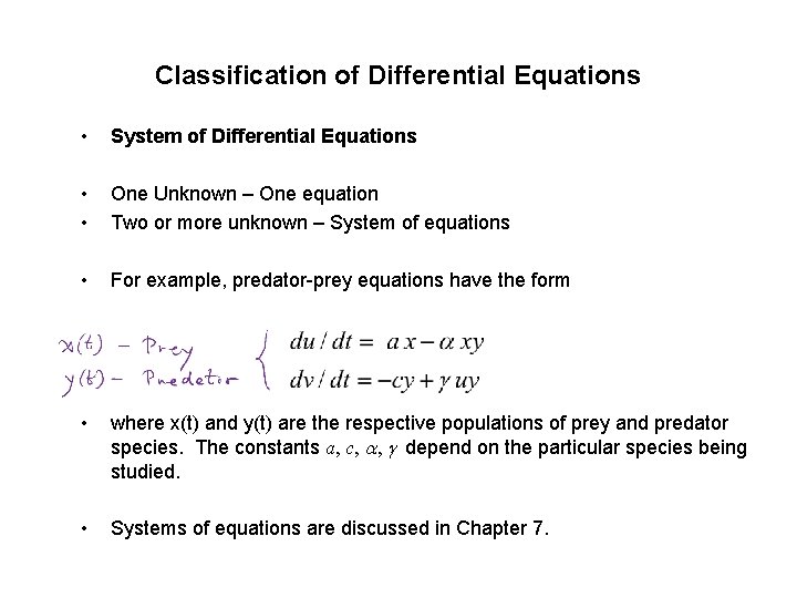
Classification of Differential Equations • System of Differential Equations • • One Unknown – One equation Two or more unknown – System of equations • For example, predator-prey equations have the form • where x(t) and y(t) are the respective populations of prey and predator species. The constants a, c, , depend on the particular species being studied. • Systems of equations are discussed in Chapter 7.

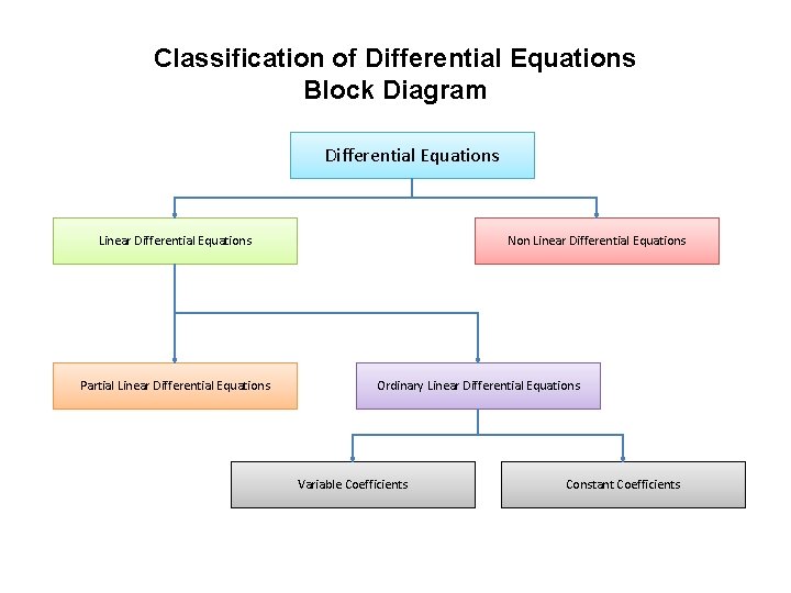
Classification of Differential Equations Block Diagram Differential Equations Linear Differential Equations Partial Linear Differential Equations Non Linear Differential Equations Ordinary Linear Differential Equations Variable Coefficients Constant Coefficients

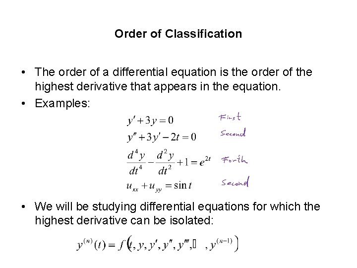
Order of Classification • The order of a differential equation is the order of the highest derivative that appears in the equation. • Examples: • We will be studying differential equations for which the highest derivative can be isolated:

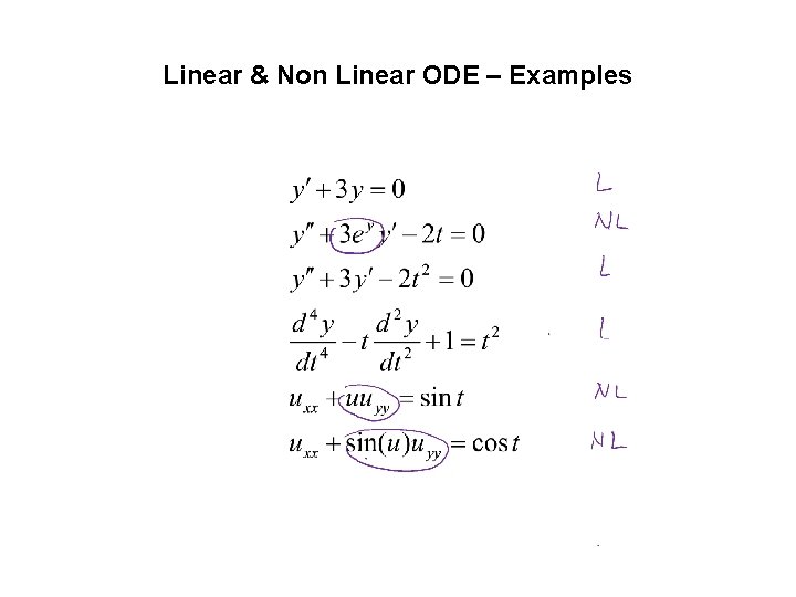
Linear & Non Linear ODE • An ordinary differential equation is linear if F is linear in the variables • Thus the general linear ODE has the form

Linear & Non Linear ODE – Examples

Linearization of a Non Linear ODE – Example

Linearization of a Non Linear ODE – Example

Linearization of a Non Linear ODE – Example

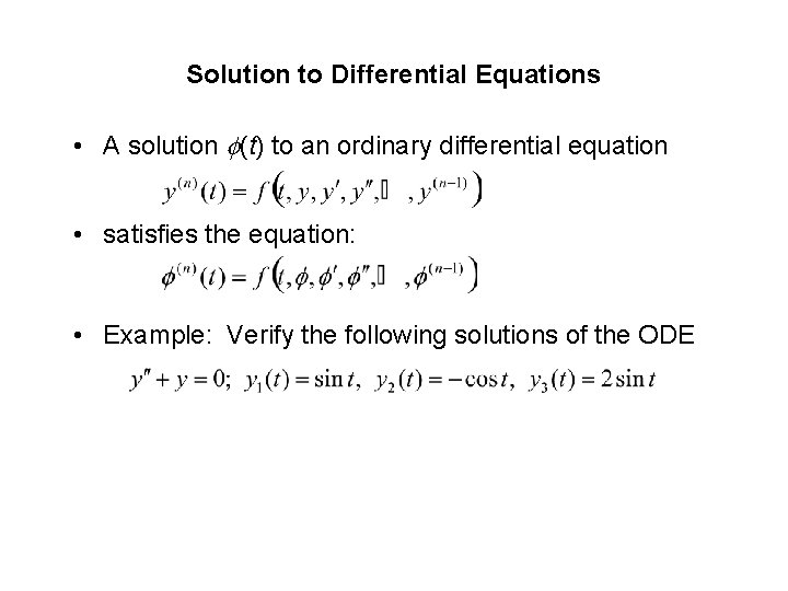
Solution to Differential Equations • A solution (t) to an ordinary differential equation • satisfies the equation: • Example: Verify the following solutions of the ODE

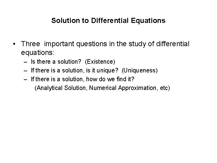
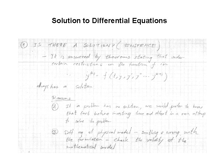
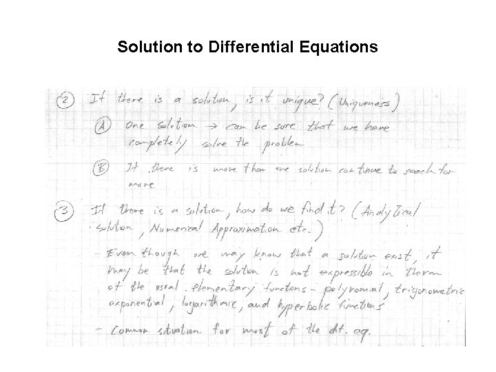
Solution to Differential Equations • Three important questions in the study of differential equations: – Is there a solution? (Existence) – If there is a solution, is it unique? (Uniqueness) – If there is a solution, how do we find it? (Analytical Solution, Numerical Approximation, etc)

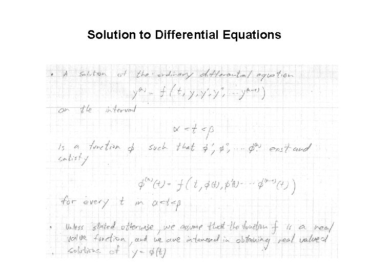
Solution to Differential Equations

Solution to Differential Equations

Solution to Differential Equations