Class 3 Estimating Scoring Rules for Sequence Alignment

Class 3: Estimating Scoring Rules for Sequence Alignment .

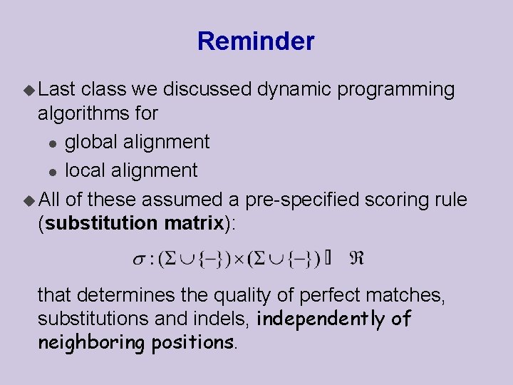
Reminder u Last class we discussed dynamic programming algorithms for l global alignment l local alignment u All of these assumed a pre-specified scoring rule (substitution matrix): that determines the quality of perfect matches, substitutions and indels, independently of neighboring positions.

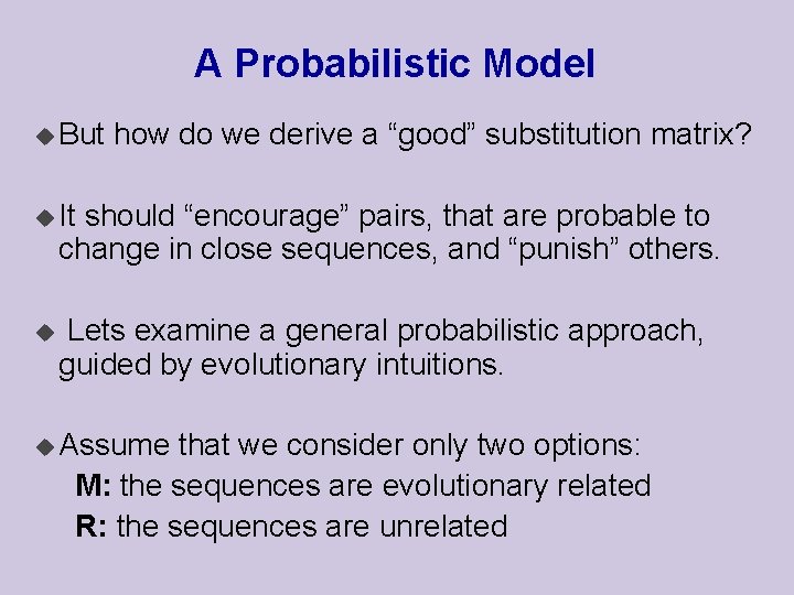
A Probabilistic Model u But how do we derive a “good” substitution matrix? u It should “encourage” pairs, that are probable to change in close sequences, and “punish” others. u Lets examine a general probabilistic approach, guided by evolutionary intuitions. u Assume that we consider only two options: M: the sequences are evolutionary related R: the sequences are unrelated

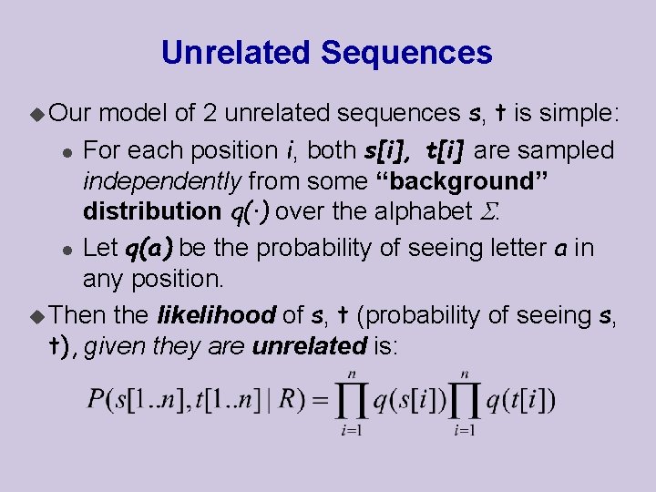
Unrelated Sequences model of 2 unrelated sequences s, t is simple: l For each position i, both s[i], t[i] are sampled independently from some “background” distribution q(·) over the alphabet . l Let q(a) be the probability of seeing letter a in any position. u Then the likelihood of s, t (probability of seeing s, t), given they are unrelated is: u Our

Related Sequences u Now lets assume that each pair of aligned positions (s[i], t[i]) evolved from a common ancestor =>s[i], t[i] are dependent ! l We assume s[i], t[i] are sampled from some distribution p(·, ·) of letters pairs. l Let p(a, b) be a probability that some ancestral letter evolved into this particular pair of letters u Then the likelihood of s, t, given they are related is:

Decision Problem two sequences s[1. . n] and t[1. . n] decide whether they were sampled from M or from R u Given u This is an instance of a decision problem that is quite frequent in statistics: hypothesis testing want to construct a procedure Decide(s, t) = D(s, t) that returns either M or R u Intuitively, we want to compare the likelihoods of the data in both models… u We

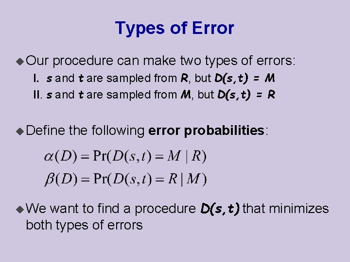
Types of Error u Our procedure can make two types of errors: I. s and t are sampled from R, but D(s, t) = M II. s and t are sampled from M, but D(s, t) = R u Define the following error probabilities: want to find a procedure D(s, t) that minimizes both types of errors u We

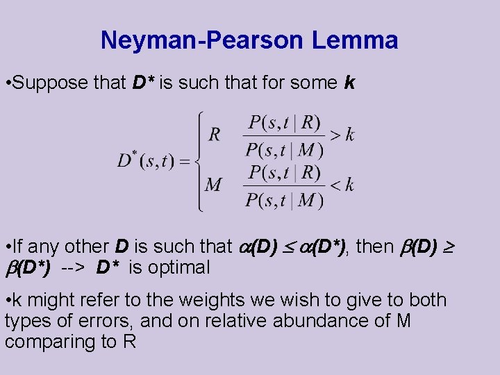
Neyman-Pearson Lemma • Suppose that D* is such that for some k • If any other D is such that (D) (D*), then (D) (D*) --> D* is optimal • k might refer to the weights we wish to give to both types of errors, and on relative abundance of M comparing to R

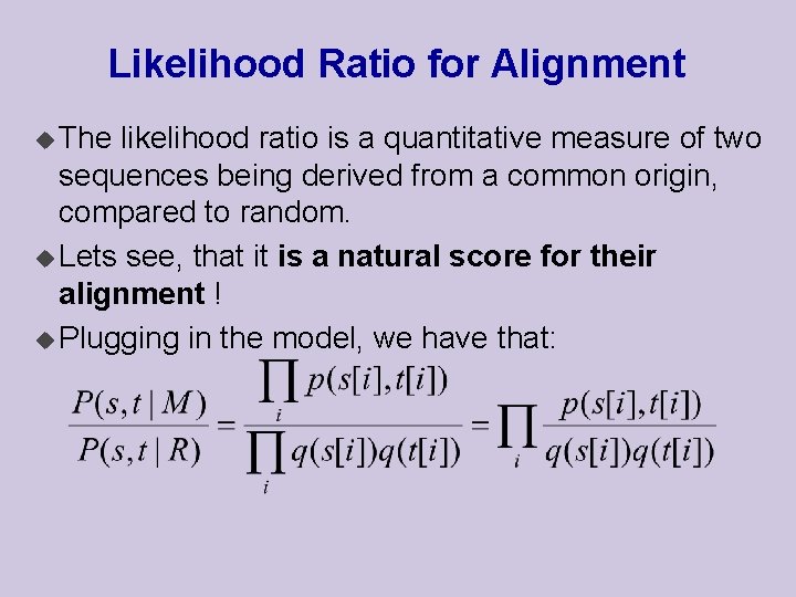
Likelihood Ratio for Alignment u The likelihood ratio is a quantitative measure of two sequences being derived from a common origin, compared to random. u Lets see, that it is a natural score for their alignment ! u Plugging in the model, we have that:

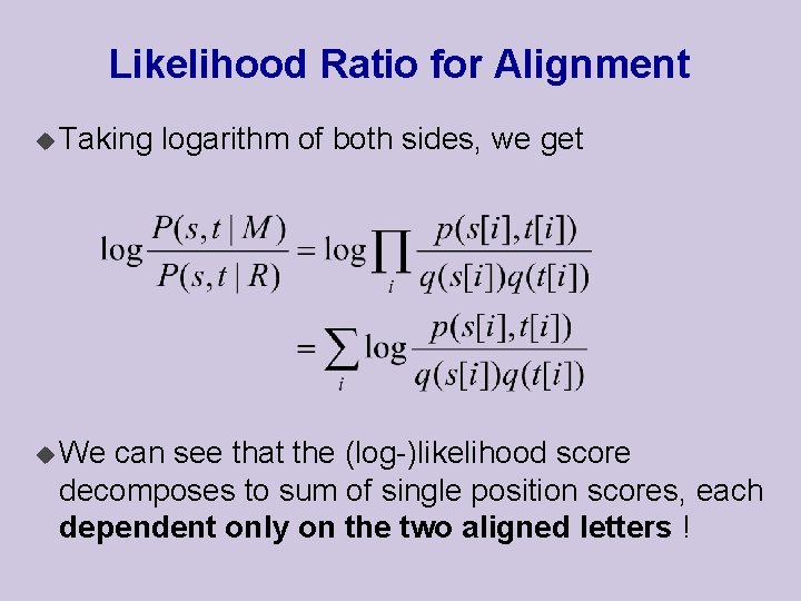
Likelihood Ratio for Alignment u Taking u We logarithm of both sides, we get can see that the (log-)likelihood score decomposes to sum of single position scores, each dependent only on the two aligned letters !

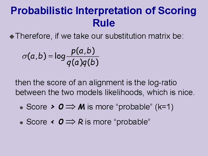
Probabilistic Interpretation of Scoring Rule u Therefore, if we take our substitution matrix be: then the score of an alignment is the log-ratio between the two models likelihoods, which is nice. l Score > 0 M is more “probable” (k=1) l Score < 0 R is more “probable”

Modeling Assumptions u It is important to note that this interpretation depends on our modeling assumption of the two hypotheses!! u For example, if we assume that the letter in each position depends on the letter in the preceding position, then the likelihood ration will have a different form.

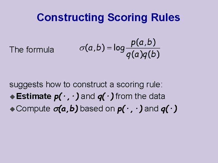
Constructing Scoring Rules The formula suggests how to construct a scoring rule: u Estimate p(·, ·) and q(·) from the data u Compute (a, b) based on p(·, ·) and q(·)

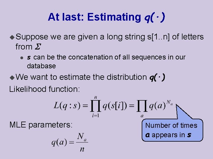
Estimating Probabilities u Suppose we are given a long string s[1. . n] of letters from u We want to estimate the distribution q(·) that “generated” the sequence u How should we go about this? u We build on theory of parameter estimation in statistics

Statistical Parameter Fitting u Consider l l l instances x[1], x[2], …, x[M] such that The set of values that x can take is known Each is sampled from the same (unknown) distribution of a known family (multinomial, Gaussian, Poisson, etc. ) Each is sampled independently of the rest task is to find a parameters set defining the most likely distribution P(x| ), from which the instances could be sampled, I. e. u The parameters depend on the given family of probability distributions. u The

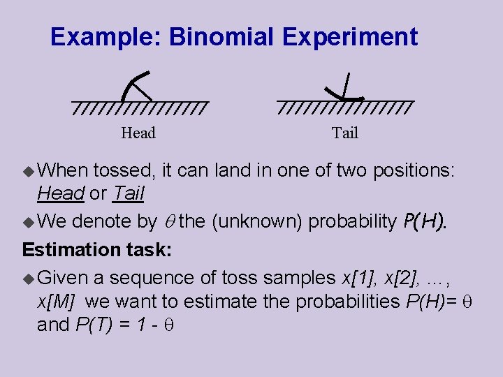
Example: Binomial Experiment Head u When Tail tossed, it can land in one of two positions: Head or Tail u We denote by the (unknown) probability P(H). Estimation task: u Given a sequence of toss samples x[1], x[2], …, x[M] we want to estimate the probabilities P(H)= and P(T) = 1 -

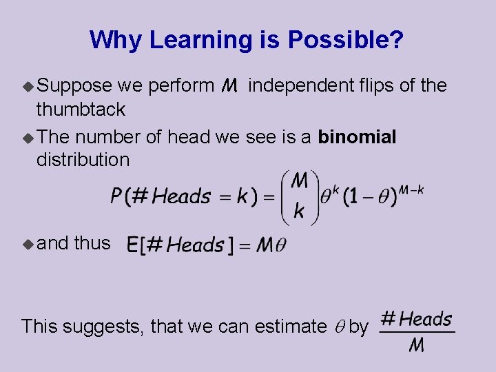
Why Learning is Possible? we perform M independent flips of the thumbtack u The number of head we see is a binomial distribution u Suppose u and thus This suggests, that we can estimate by

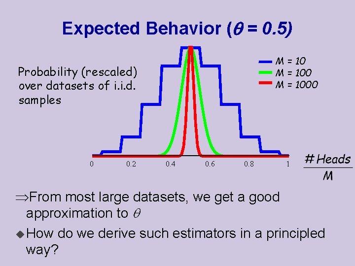
Expected Behavior ( = 0. 5) M = 1000 Probability (rescaled) over datasets of i. i. d. samples 0 0. 2 0. 4 0. 6 0. 8 1 From most large datasets, we get a good approximation to u How do we derive such estimators in a principled way?

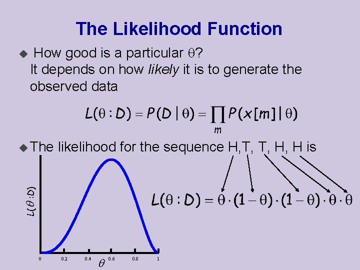
The Likelihood Function u How good is a particular ? It depends on how likely it is to generate the observed data likelihood for the sequence H, T, T, H, H is L( : D) u The 0 0. 2 0. 4 0. 6 0. 8 1

Maximum Likelihood Estimation u MLE Principle: Learn parameters that maximize the likelihood function u This is one of the most commonly used estimators in statistics u Intuitively appealing

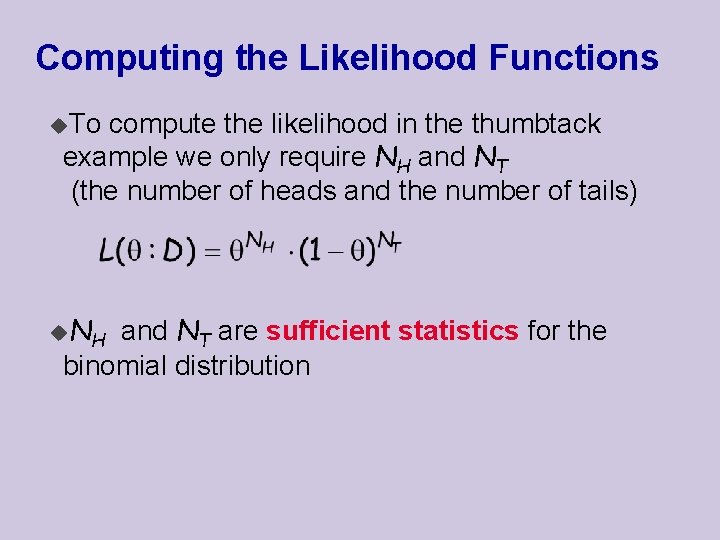
Computing the Likelihood Functions u. To compute the likelihood in the thumbtack example we only require NH and NT (the number of heads and the number of tails) u. N H and NT are sufficient statistics for the binomial distribution

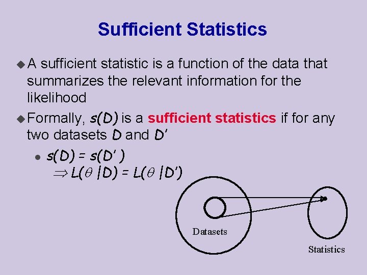
Sufficient Statistics u. A sufficient statistic is a function of the data that summarizes the relevant information for the likelihood u Formally, s(D) is a sufficient statistics if for any two datasets D and D’ l s(D) = s(D’ ) L( |D) = L( |D’) Datasets Statistics

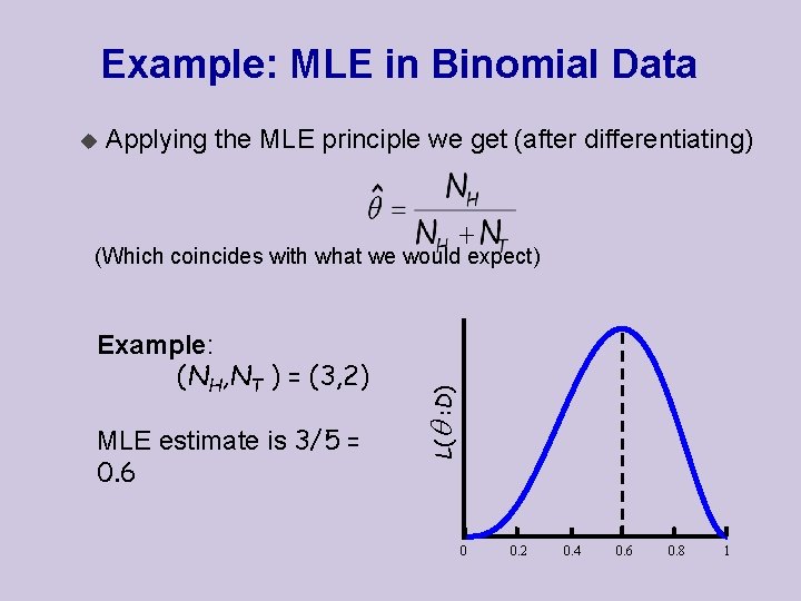
Example: MLE in Binomial Data u Applying the MLE principle we get (after differentiating) Example: (NH, NT ) = (3, 2) MLE estimate is 3/5 = 0. 6 L( : D) (Which coincides with what we would expect) 0 0. 2 0. 4 0. 6 0. 8 1

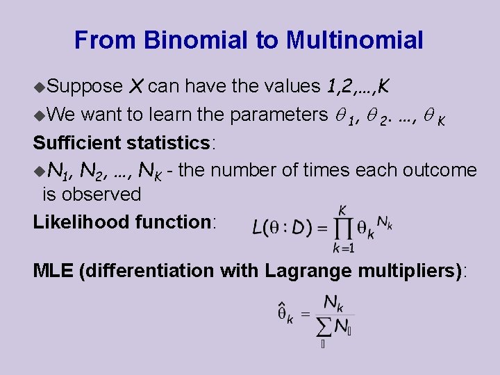
From Binomial to Multinomial X can have the values 1, 2, …, K u. We want to learn the parameters 1, 2. …, K Sufficient statistics: u. N 1, N 2, …, NK - the number of times each outcome is observed Likelihood function: u. Suppose MLE (differentiation with Lagrange multipliers):

At last: Estimating q(·) u Suppose from l we are given a long string s[1. . n] of letters s can be the concatenation of all sequences in our database want to estimate the distribution q(·) Likelihood function: u We MLE parameters: Number of times a appears in s

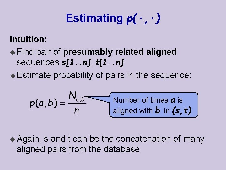
Estimating p(·, ·) Intuition: u Find pair of presumably related aligned sequences s[1. . n], t[1. . n] u Estimate probability of pairs in the sequence: Number of times a is aligned with b in (s, t) u Again, s and t can be the concatenation of many aligned pairs from the database

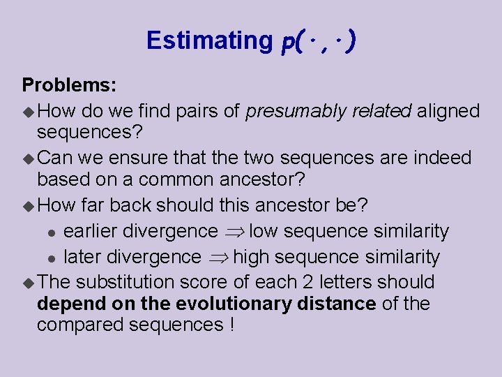
Estimating p(·, ·) Problems: u How do we find pairs of presumably related aligned sequences? u Can we ensure that the two sequences are indeed based on a common ancestor? u How far back should this ancestor be? l earlier divergence low sequence similarity l later divergence high sequence similarity u The substitution score of each 2 letters should depend on the evolutionary distance of the compared sequences !

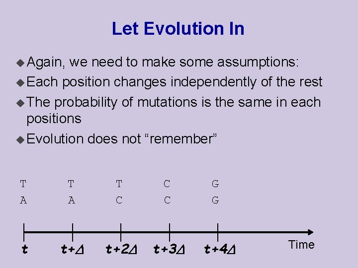
Let Evolution In u Again, we need to make some assumptions: u Each position changes independently of the rest u The probability of mutations is the same in each positions u Evolution does not “remember” T A T C C C t t+ t+2 t+3 G G t+4 Time

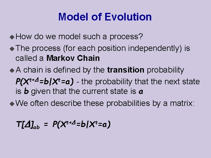
Model of Evolution u How do we model such a process? u The process (for each position independently) is called a Markov Chain u A chain is defined by the transition probability P(Xt+ =b|Xt=a) - the probability that the next state is b given that the current state is a u We often describe these probabilities by a matrix: T[ ]ab = P(Xt+ =b|Xt=a)

Two-Step Changes on T[ ], we can compute the probabilities of changes over two time periods u Based u Thus u By T[2 ] = T[ ] induction: T[k ] = T[ ] k

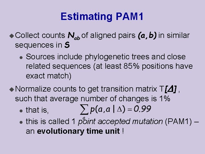
Longer Term Changes Idea: u Estimate T[ ] from some closely related sequences set S T[ ] to compute T[k ] u Derive substitution probability after time k : u Use l Note, that the score depends on evolutionary distance, as requested

Estimating PAM 1 counts Nab of aligned pairs (a, b) in similar sequences in S l Sources include phylogenetic trees and close related sequences (at least 85% positions have exact match) u Collect counts to get transition matrix T[ ] , such that average number of changes is 1% l that is, l this is called 1 point accepted mutation (PAM 1) – an evolutionary time unit ! u Normalize

Using PAM u The matrix PAM-k is defined to be the score based on Tk u Historically researchers use PAM 250 l Longer than 100 ! u Original PAM matrices were based on small number of proteins u Later versions of PAM use more examples u Used to be the most popular scoring rule

Problems with PAM u PAM extrapolates statistics collected from closely related sequences onto distant ones. u But “short-time” substitutions behave differently than “long-time” substitutions: l short-time substitutions are dominated by a single nucleotide changes that led to different translation (like L->I) l long-time substitutions dominated do not exhibit such behavior, are much more random. u Therefore, statistics would be different for different stages in evolution.

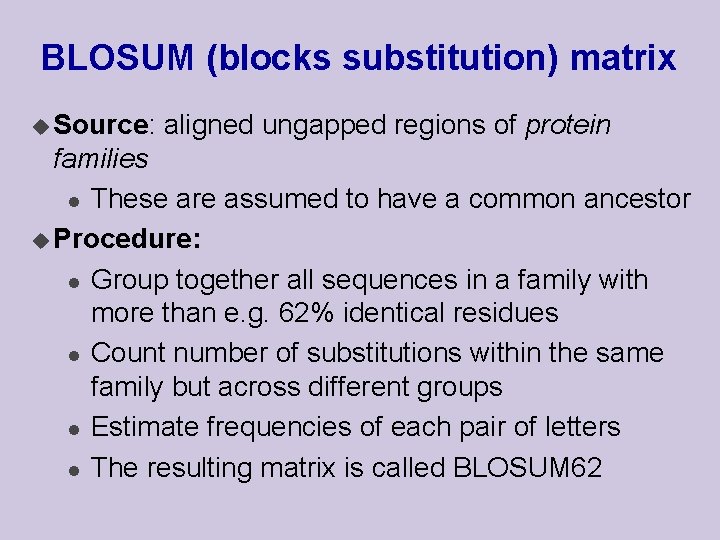
BLOSUM (blocks substitution) matrix u Source: aligned ungapped regions of protein families l These are assumed to have a common ancestor u Procedure: l Group together all sequences in a family with more than e. g. 62% identical residues l Count number of substitutions within the same family but across different groups l Estimate frequencies of each pair of letters l The resulting matrix is called BLOSUM 62