CIS 700 Advanced Machine Learning for NLP Review

CIS 700 Advanced Machine Learning for NLP Review 1: Supervised Learning, Binary Classifiers Dan Roth Department of Computer and Information Science University of Pennsylvania Augmented and modified by Vivek Srikumar Page 1

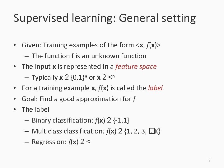
Supervised learning: General setting • Given: Training examples of the form <x, f(x)> – The function f is an unknown function • The input x is represented in a feature space – Typically x 2 {0, 1}n or x 2 <n • For a training example x, f(x) is called the label • Goal: Find a good approximation for f • The label – Binary classification: f(x) 2 {-1, 1} – Multiclassification: f(x) 2 {1, 2, 3, � , K} – Regression: f(x) 2 < 2

Nature of applications • Humans can perform a task, but can’t describe how they do it – Eg: Object detection in images – Context Sensitive Spelling • The desired function is hard to obtain in closed form – Eg: Stock market – The subject argument of a verb 3

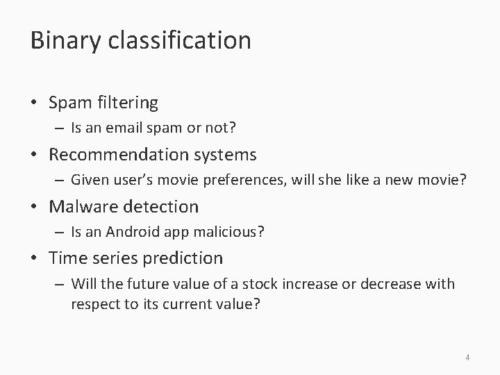
Binary classification • Spam filtering – Is an email spam or not? • Recommendation systems – Given user’s movie preferences, will she like a new movie? • Malware detection – Is an Android app malicious? • Time series prediction – Will the future value of a stock increase or decrease with respect to its current value? 4

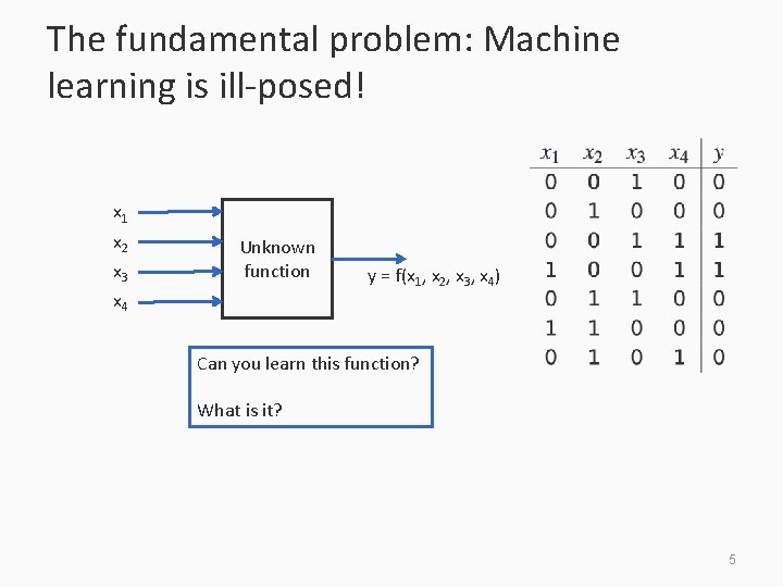
The fundamental problem: Machine learning is ill-posed! x 1 x 2 x 3 Unknown function x 4 y = f(x 1, x 2, x 3, x 4) Can you learn this function? What is it? 5

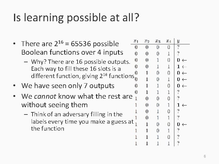
Is learning possible at all? • There are 216 = 65536 possible Boolean functions over 4 inputs – Why? There are 16 possible outputs. Each way to fill these 16 slots is a different function, giving 216 functions. • We have seen only 7 outputs • We cannot know what the rest are without seeing them – Think of an adversary filling in the labels every time you make a guess at the function 6

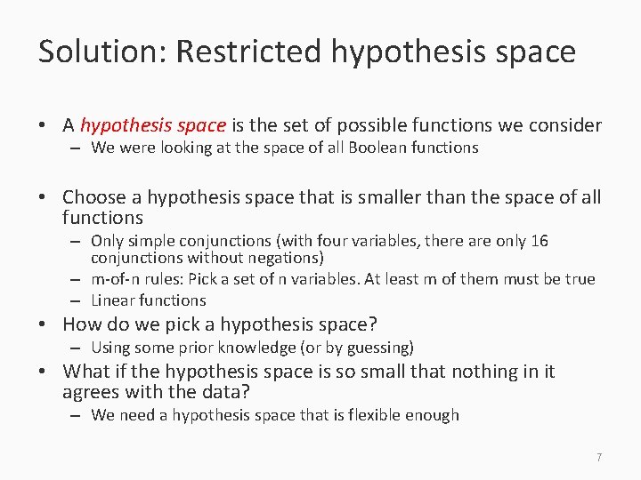
Solution: Restricted hypothesis space • A hypothesis space is the set of possible functions we consider – We were looking at the space of all Boolean functions • Choose a hypothesis space that is smaller than the space of all functions – Only simple conjunctions (with four variables, there are only 16 conjunctions without negations) – m-of-n rules: Pick a set of n variables. At least m of them must be true – Linear functions • How do we pick a hypothesis space? – Using some prior knowledge (or by guessing) • What if the hypothesis space is so small that nothing in it agrees with the data? – We need a hypothesis space that is flexible enough 7

Where are we? 1. 2. 3. 4. 5. 6. Supervised learning: The general setting Linear classifiers The Perceptron algorithm Learning as optimization Support vector machines Logistic Regression 8

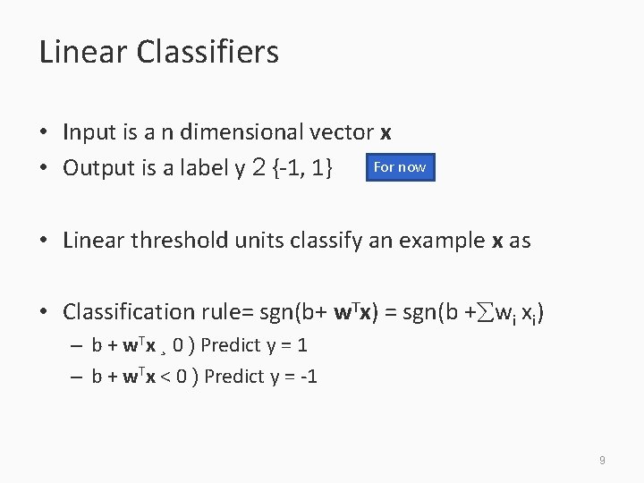
Linear Classifiers • Input is a n dimensional vector x For now • Output is a label y 2 {-1, 1} • Linear threshold units classify an example x as • Classification rule= sgn(b+ w. Tx) = sgn(b + wi xi) – b + w. Tx ¸ 0 ) Predict y = 1 – b + w. Tx < 0 ) Predict y = -1 9

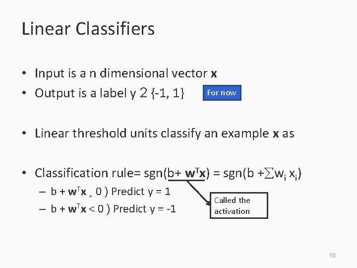
Linear Classifiers • Input is a n dimensional vector x For now • Output is a label y 2 {-1, 1} • Linear threshold units classify an example x as • Classification rule= sgn(b+ w. Tx) = sgn(b + wi xi) – b + w. Tx ¸ 0 ) Predict y = 1 – b + w. Tx < 0 ) Predict y = -1 Called the activation 10

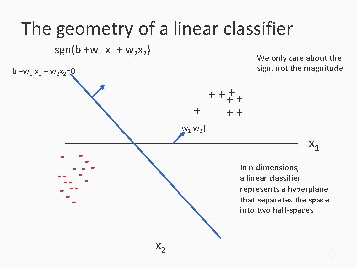
The geometry of a linear classifier sgn(b +w 1 x 1 + w 2 x 2) We only care about the sign, not the magnitude b +w 1 x 1 + w 2 x 2=0 + + ++ [w 1 w 2] - -- -- - x 1 In n dimensions, a linear classifier represents a hyperplane that separates the space into two half-spaces x 2 11

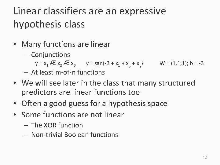
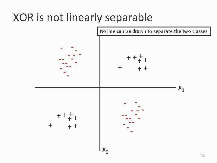
Linear classifiers are an expressive hypothesis class • Many functions are linear – Conjunctions y = x 1 Æ x 2 Æ x 3 y = sgn(-3 + x 1 + x 2 + x 3) W = (1, 1, 1); b = -3 – At least m-of-n functions • We will see later in the class that many structured predictors are linear functions too • Often a good guess for a hypothesis space • Some functions are not linear – The XOR function – Non-trivial Boolean functions 12

XOR is not linearly separable No line can be drawn to separate the two classes - -- -- - + + ++ x 1 - -- -- - + + ++ x 2 13

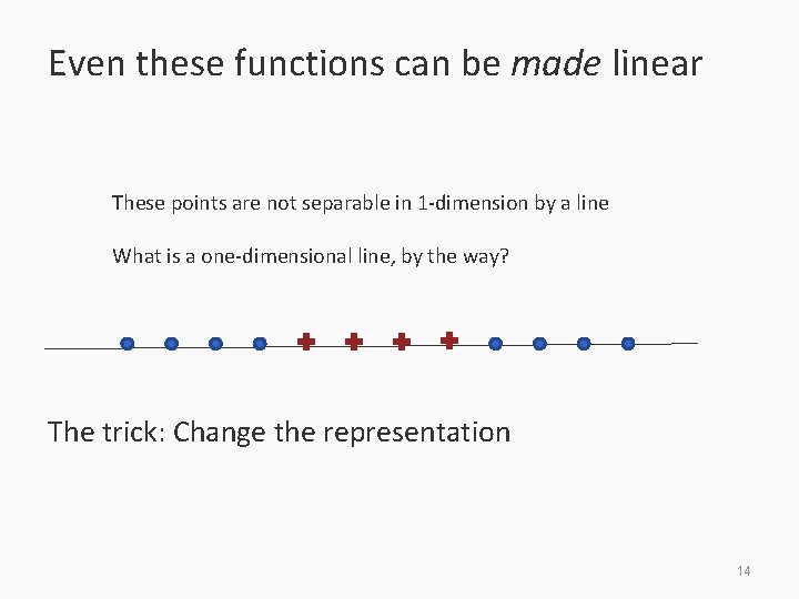
Even these functions can be made linear These points are not separable in 1 -dimension by a line What is a one-dimensional line, by the way? The trick: Change the representation 14

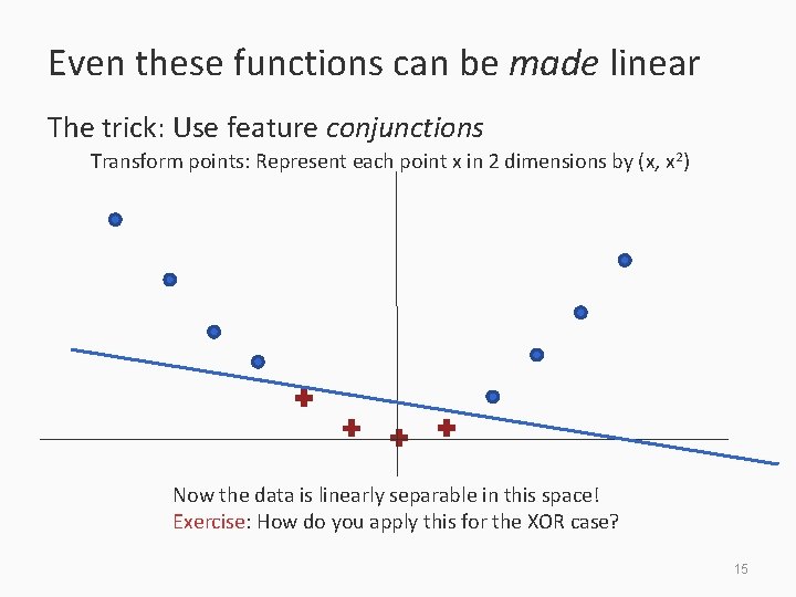
Even these functions can be made linear The trick: Use feature conjunctions Transform points: Represent each point x in 2 dimensions by (x, x 2) Now the data is linearly separable in this space! Exercise: How do you apply this for the XOR case? 15

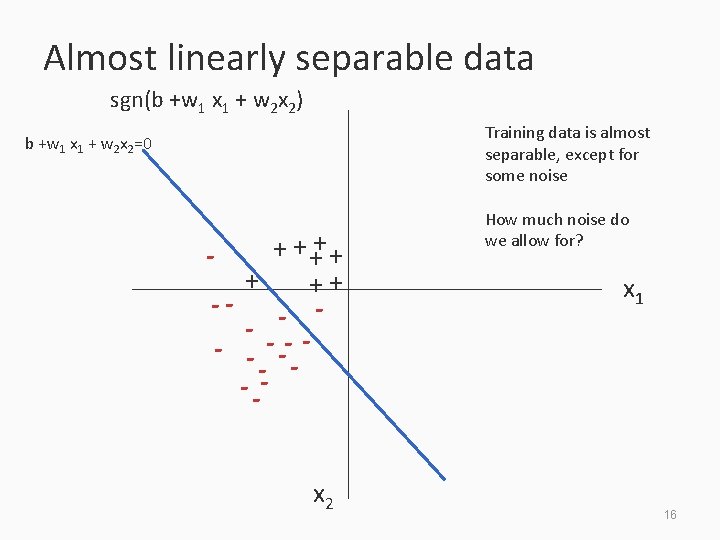
Almost linearly separable data sgn(b +w 1 x 1 + w 2 x 2) Training data is almost separable, except for some noise b +w 1 x 1 + w 2 x 2=0 + ++ -- - - -- -- -x 2 How much noise do we allow for? x 1 16

Training a linear classifier Three cases to consider: 1. Training data is linearly separable – Simple conjunctions, general linear functions, etc 2. Training data is linearly inseparable – XOR, etc 3. Training data is almost linearly separable – – Noise in the data We could allow some the classifier to make some mistakes on the training data to account for these 17

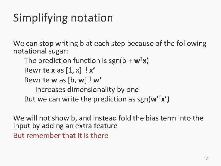
Simplifying notation We can stop writing b at each step because of the following notational sugar: The prediction function is sgn(b + w. Tx) Rewrite x as [1, x] ! x’ Rewrite w as [b, w] ! w’ increases dimensionality by one But we can write the prediction as sgn(w’Tx’) We will not show b, and instead fold the bias term into the input by adding an extra feature But remember that it is there 18

Where are we? 1. 2. 3. 4. 5. 6. Supervised learning: The general setting Linear classifiers The Perceptron algorithm Learning as optimization Support vector machines Logistic Regression 19

The Perceptron algorithm • Rosenblatt 1958 • The goal is to find a separating hyperplane – For separable data, guaranteed to find one • An online algorithm – Processes one example at a time • Several variants exist (will discuss briefly at towards the end) 20

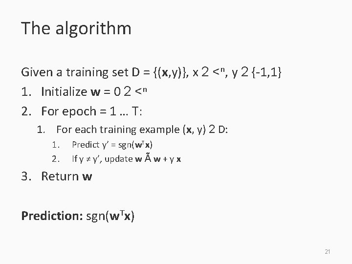
The algorithm Given a training set D = {(x, y)}, x 2 <n, y 2 {-1, 1} 1. Initialize w = 0 2 <n 2. For epoch = 1 … T: 1. For each training example (x, y) 2 D: 1. 2. Predict y’ = sgn(w. Tx) If y ≠ y’, update w à w + y x 3. Return w Prediction: sgn(w. Tx) 21

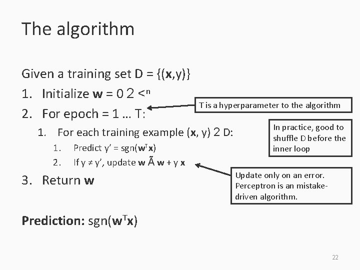
The algorithm Given a training set D = {(x, y)} 1. Initialize w = 0 2 <n 2. For epoch = 1 … T: T is a hyperparameter to the algorithm 1. For each training example (x, y) 2 D: 1. 2. Predict y’ = sgn(w. Tx) If y ≠ y’, update w à w + y x 3. Return w In practice, good to shuffle D before the inner loop Update only on an error. Perceptron is an mistakedriven algorithm. Prediction: sgn(w. Tx) 22

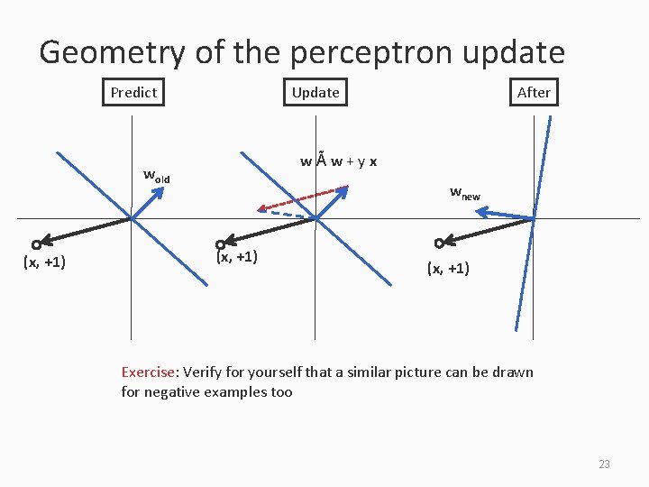
Geometry of the perceptron update Predict Update wÃw+yx wold (x, +1) After wnew (x, +1) Exercise: Verify for yourself that a similar picture can be drawn for negative examples too 23

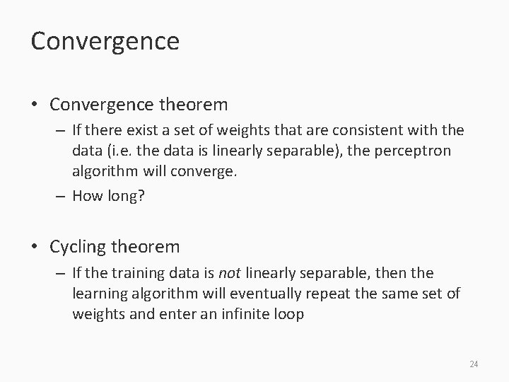
Convergence • Convergence theorem – If there exist a set of weights that are consistent with the data (i. e. the data is linearly separable), the perceptron algorithm will converge. – How long? • Cycling theorem – If the training data is not linearly separable, then the learning algorithm will eventually repeat the same set of weights and enter an infinite loop 24

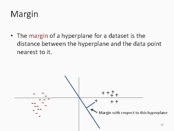
Margin • The margin of a hyperplane for a dataset is the distance between the hyperplane and the data point nearest to it. - -- -- - + + ++ Margin with respect to this hyperplane 25

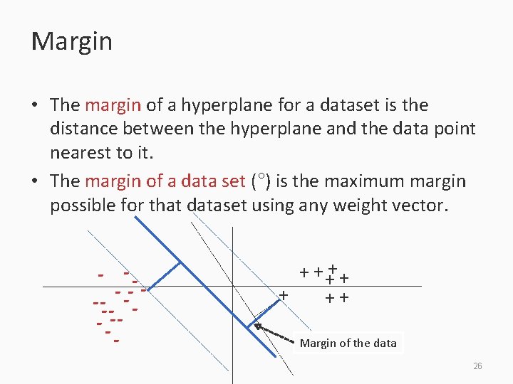
Margin • The margin of a hyperplane for a dataset is the distance between the hyperplane and the data point nearest to it. • The margin of a data set (°) is the maximum margin possible for that dataset using any weight vector. - -- -- - + + ++ Margin of the data 26

The mistake bound theorem [Novikoff 1962] Let D={(xi, yi)} be a labeled dataset that is separable Let ||xi||· R for all examples. Let ° be the margin of the dataset D. Then, the perceptron algorithm will make at most R 2/° 2 mistakes on the data. Proof idea: We know that there is some true weight vector w*. Each perceptron update reduces the angle between w and w*. Note: The theorem doesn’t depend on the number of examples we have. 27

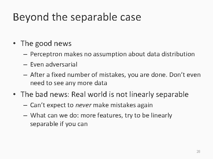
Beyond the separable case • The good news – Perceptron makes no assumption about data distribution – Even adversarial – After a fixed number of mistakes, you are done. Don’t even need to see any more data • The bad news: Real world is not linearly separable – Can’t expect to never make mistakes again – What can we do: more features, try to be linearly separable if you can 28

Variants of the algorithm • So far: We return the final weight vector • Averaged perceptron – Remember every weight vector in your sequence of updates. – Weigh each weight vector as a function of the number of examples that survived this weight vector. – Make a prediction with the weighted average of the weight vectors. – Comes with strong theoretical guarantees about generalization. – Need to be smart about implementation. 29

Next steps • What is the perceptron doing? – Error-bound exists, but over training data – Is it minimizing a loss function? Can we say something about future errors? • More on different loss functions • Support vector machine – A look at regularization • Logistic Regression 30