CIS 700 Advanced Machine Learning for NLP Review

CIS 700 Advanced Machine Learning for NLP Review 2: Loss minimization, SVM and Logistic Regression Dan Roth Department of Computer and Information Science University of Pennsylvania Augmented and modified by Vivek Srikumar Page 1

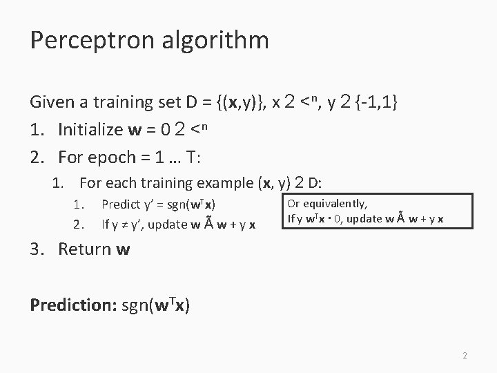
Perceptron algorithm Given a training set D = {(x, y)}, x 2 <n, y 2 {-1, 1} 1. Initialize w = 0 2 <n 2. For epoch = 1 … T: 1. For each training example (x, y) 2 D: 1. 2. Predict y’ = sgn(w. Tx) If y ≠ y’, update w à w + y x Or equivalently, If y w. Tx · 0, update w à w + y x 3. Return w Prediction: sgn(w. Tx) 2

Where are we? 1. 2. 3. 4. 5. 6. Supervised learning: The general setting Linear classifiers The Perceptron algorithm Support vector machines Learning as optimization Logistic Regression 3

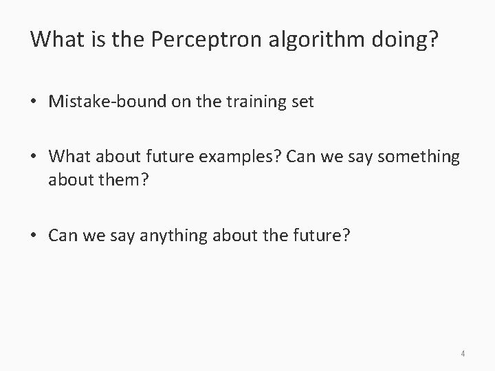
What is the Perceptron algorithm doing? • Mistake-bound on the training set • What about future examples? Can we say something about them? • Can we say anything about the future? 4

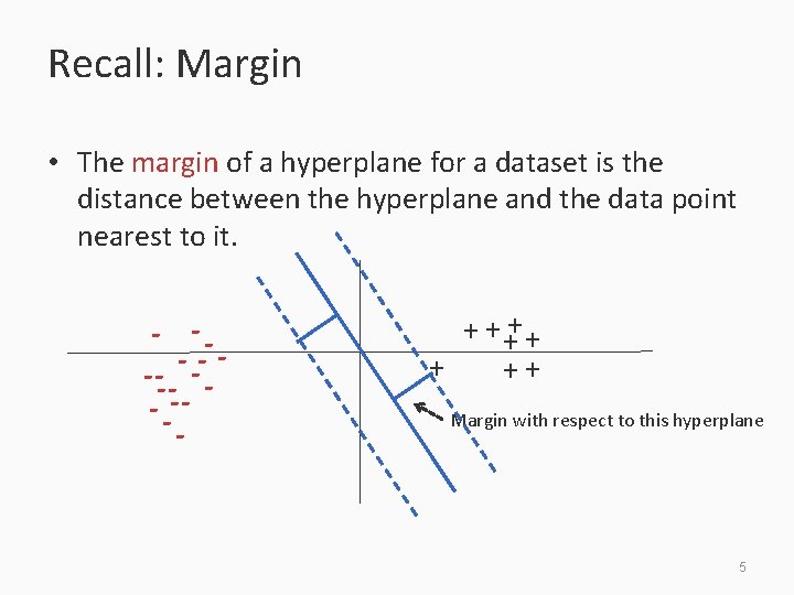
Recall: Margin • The margin of a hyperplane for a dataset is the distance between the hyperplane and the data point nearest to it. - -- -- - + + ++ Margin with respect to this hyperplane 5

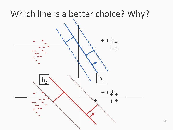
Which line is a better choice? Why? - -- -- - - -- h 2 - -- -- - + + ++ h 1 + + ++ 6

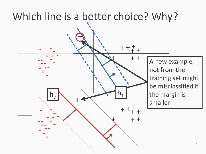
Which line is a better choice? Why? + ++ + + ++ - -- -- - - -- h 2 - -- -- - + h 1 + + ++ A new example, not from the training set might be misclassified if the margin is smaller 7

Maximal margin and generalization • Larger margin gives better generalization • Note: learning is done on a training set – You can minimize your performance on the training data – But, you care about your performance on previousely unseen data • The notion of a margin is related to the notion of the expressivity of the hypothesis space – In this case, a hypothesis space of linear functions • Maximizing margin => fewer errors on future examples – This idea forms the basis of many learning algorithms • SVM, averaged perceptron, Ada. Boost, … 8

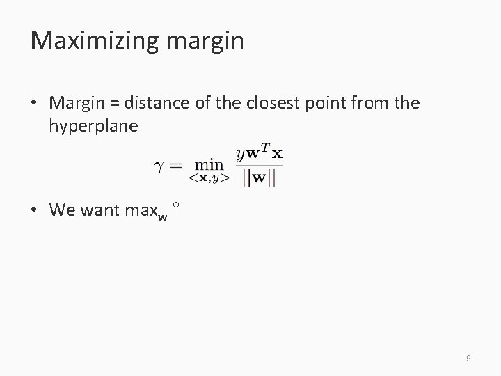
Maximizing margin • Margin = distance of the closest point from the hyperplane • We want maxw ° 9

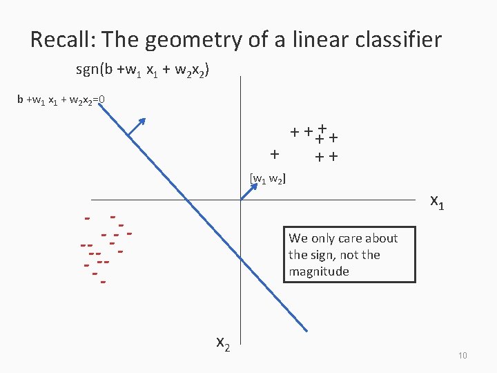
Recall: The geometry of a linear classifier sgn(b +w 1 x 1 + w 2 x 2) b +w 1 x 1 + w 2 x 2=0 + + ++ [w 1 w 2] - -- -- - x 1 We only care about the sign, not the magnitude x 2 10

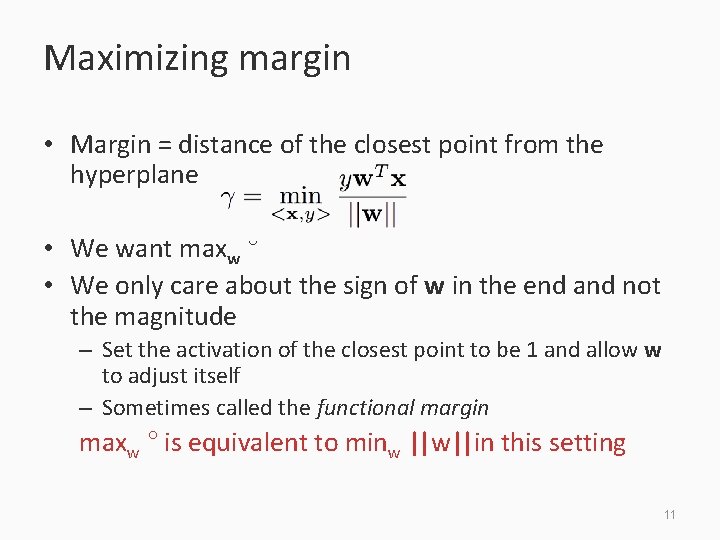
Maximizing margin • Margin = distance of the closest point from the hyperplane • We want maxw ° • We only care about the sign of w in the end and not the magnitude – Set the activation of the closest point to be 1 and allow w to adjust itself – Sometimes called the functional margin maxw ° is equivalent to minw ||w||in this setting 11

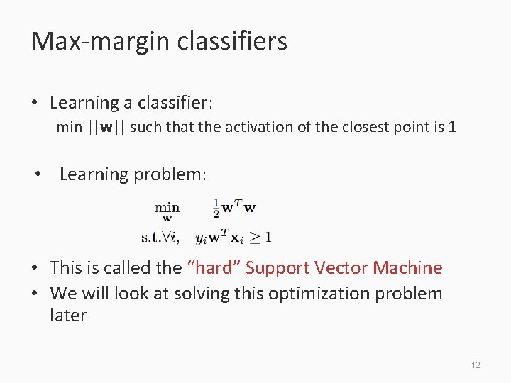
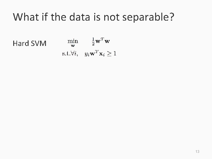
Max-margin classifiers • Learning a classifier: min ||w|| such that the activation of the closest point is 1 • Learning problem: • This is called the “hard” Support Vector Machine • We will look at solving this optimization problem later 12

What if the data is not separable? Hard SVM 13

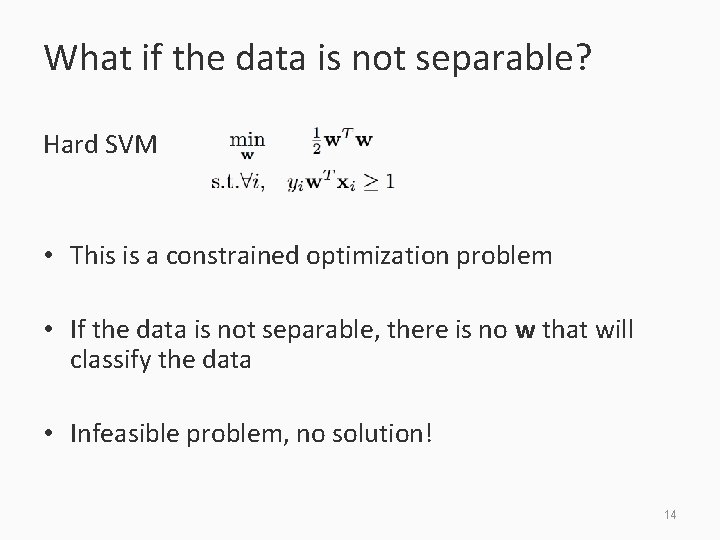
What if the data is not separable? Hard SVM • This is a constrained optimization problem • If the data is not separable, there is no w that will classify the data • Infeasible problem, no solution! 14

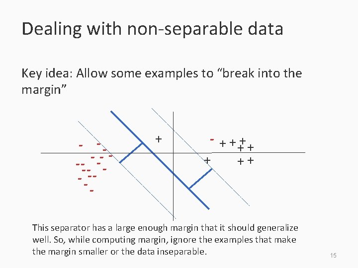
Dealing with non-separable data Key idea: Allow some examples to “break into the margin” - -- -- - +++ ++ This separator has a large enough margin that it should generalize well. So, while computing margin, ignore the examples that make the margin smaller or the data inseparable. 15

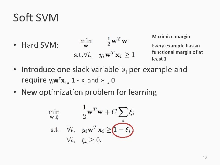
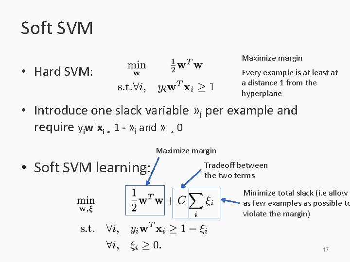
Soft SVM • Hard SVM: Maximize margin Every example has an functional margin of at least 1 • Introduce one slack variable » i per example and require yiw. Txi ¸ 1 - » i and » i ¸ 0 • New optimization problem for learning 16

Soft SVM Maximize margin • Hard SVM: Every example is at least at a distance 1 from the hyperplane • Introduce one slack variable » i per example and require yiw. Txi ¸ 1 - » i and » i ¸ 0 Maximize margin • Soft SVM learning: Tradeoff between the two terms Minimize total slack (i. e allow as few examples as possible to violate the margin) 17

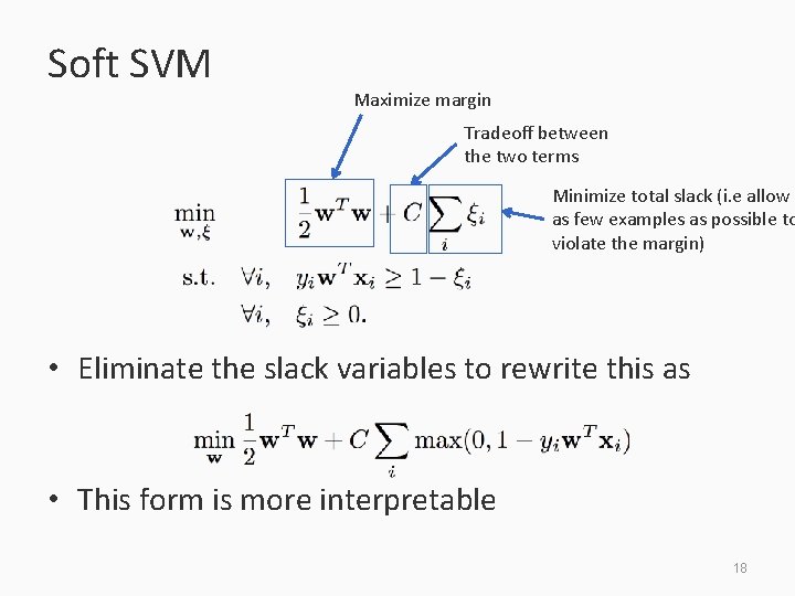
Soft SVM Maximize margin Tradeoff between the two terms Minimize total slack (i. e allow as few examples as possible to violate the margin) • Eliminate the slack variables to rewrite this as • This form is more interpretable 18

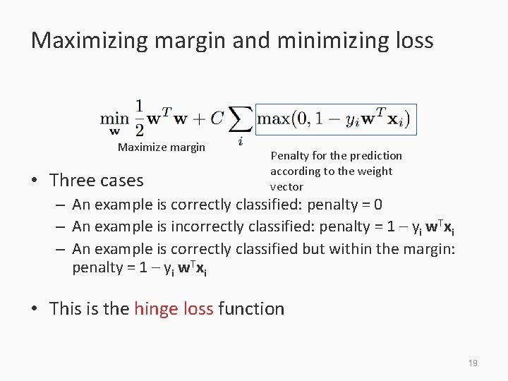
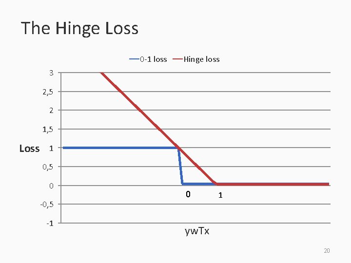
Maximizing margin and minimizing loss Maximize margin • Three cases Penalty for the prediction according to the weight vector – An example is correctly classified: penalty = 0 – An example is incorrectly classified: penalty = 1 – yi w. Txi – An example is correctly classified but within the margin: penalty = 1 – yi w. Txi • This is the hinge loss function 19

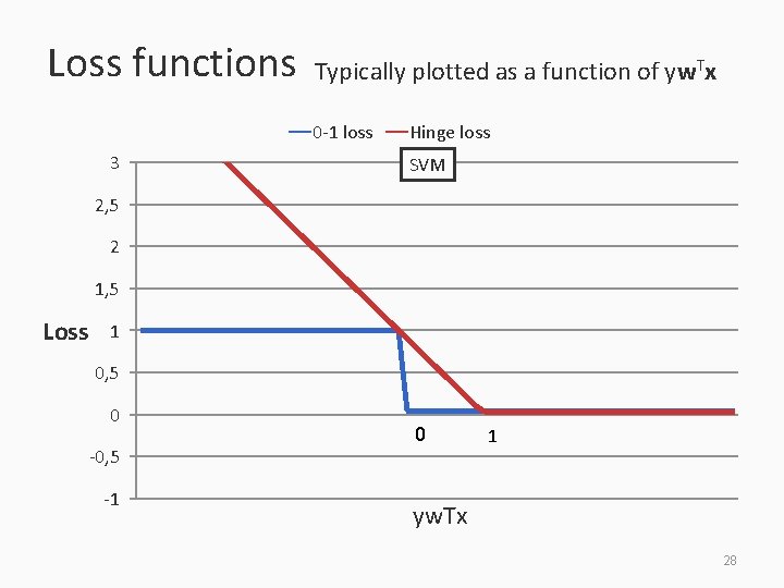
The Hinge Loss 0 -1 loss Hinge loss 3 2, 5 2 1, 5 Loss 1 0, 5 0 -0, 5 -1 0 1 yw. Tx 20

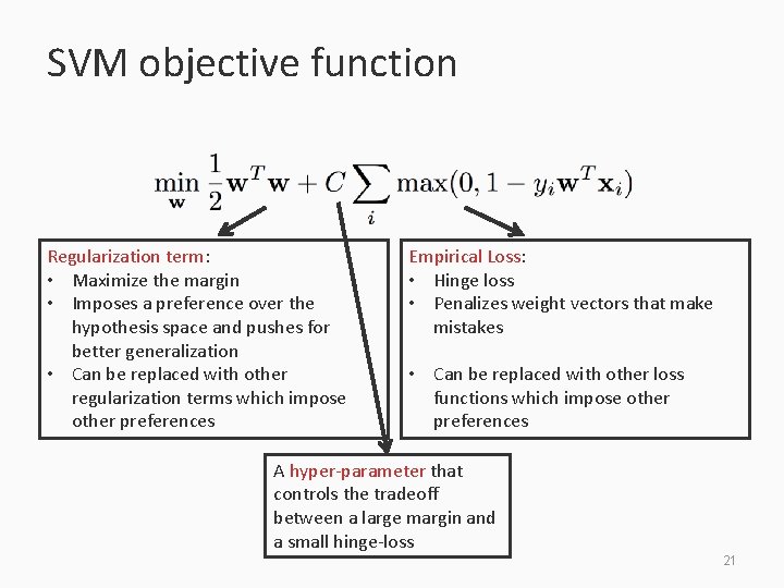
SVM objective function Regularization term: • Maximize the margin • Imposes a preference over the hypothesis space and pushes for better generalization • Can be replaced with other regularization terms which impose other preferences Empirical Loss: • Hinge loss • Penalizes weight vectors that make mistakes • Can be replaced with other loss functions which impose other preferences A hyper-parameter that controls the tradeoff between a large margin and a small hinge-loss 21

Where are we? 1. 2. 3. 4. 5. 6. Supervised learning: The general setting Linear classifiers The Perceptron algorithm Support vector machines Learning as optimization Logistic Regression 22

Computational Learning Theory • Studies theoretical issues about the importance of representation, sample complexity (how many examples are enough), computational complexity (how fast can I learn) – Led to algorithms such as support vector machine and boosting • No assumptions about the distribution of examples – But assume that both training and test examples come from the same distribution • Provides bounds that depend on the size of the hypothesis class 23

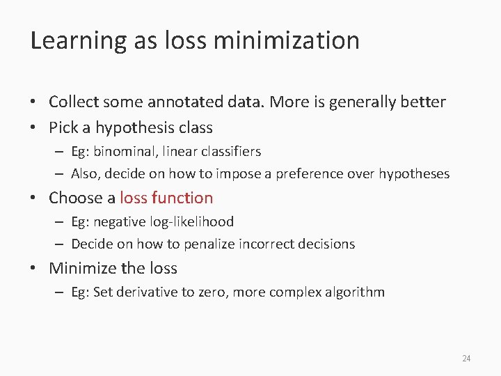
Learning as loss minimization • Collect some annotated data. More is generally better • Pick a hypothesis class – Eg: binominal, linear classifiers – Also, decide on how to impose a preference over hypotheses • Choose a loss function – Eg: negative log-likelihood – Decide on how to penalize incorrect decisions • Minimize the loss – Eg: Set derivative to zero, more complex algorithm 24

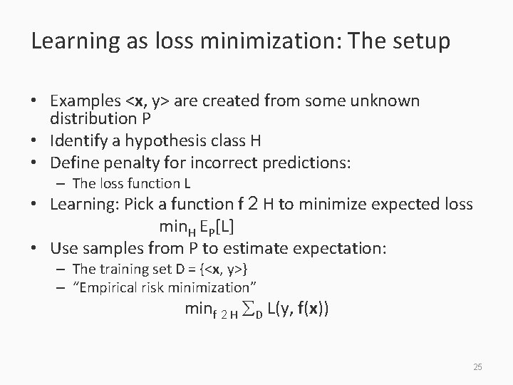
Learning as loss minimization: The setup • Examples <x, y> are created from some unknown distribution P • Identify a hypothesis class H • Define penalty for incorrect predictions: – The loss function L • Learning: Pick a function f 2 H to minimize expected loss min. H EP[L] • Use samples from P to estimate expectation: – The training set D = {<x, y>} – “Empirical risk minimization” minf 2 H D L(y, f(x)) 25

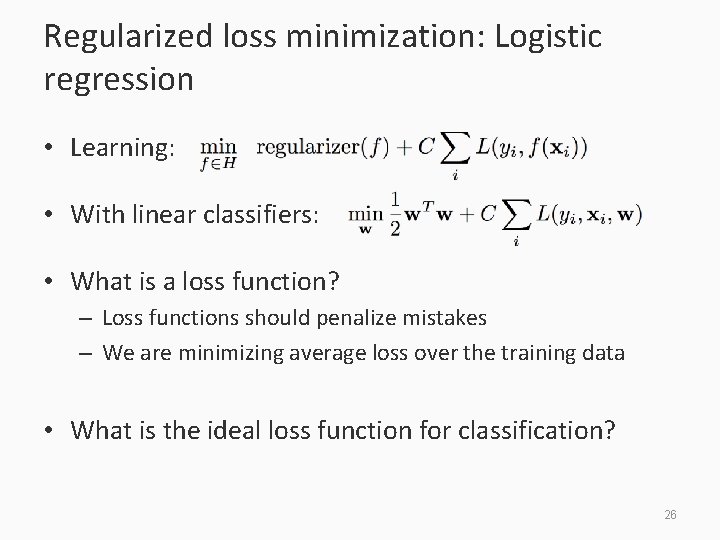
Regularized loss minimization: Logistic regression • Learning: • With linear classifiers: • What is a loss function? – Loss functions should penalize mistakes – We are minimizing average loss over the training data • What is the ideal loss function for classification? 26

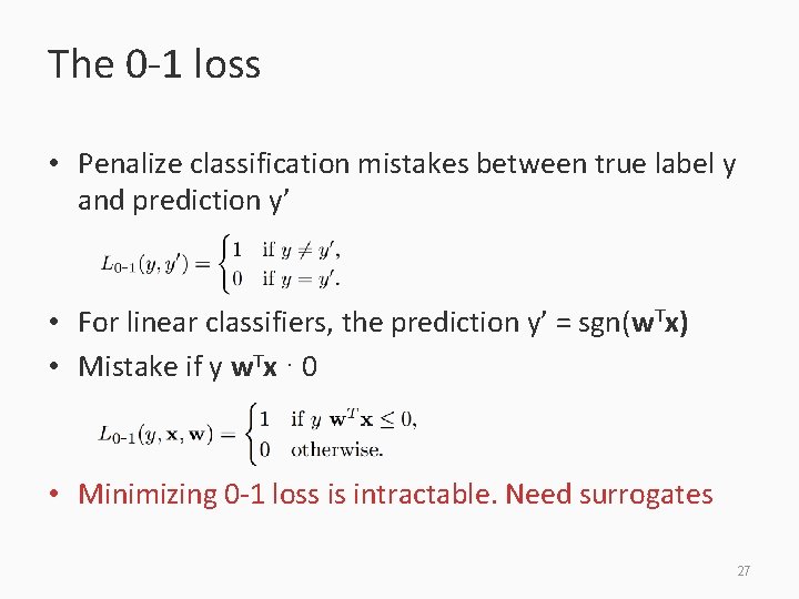
The 0 -1 loss • Penalize classification mistakes between true label y and prediction y’ • For linear classifiers, the prediction y’ = sgn(w. Tx) • Mistake if y w. Tx · 0 • Minimizing 0 -1 loss is intractable. Need surrogates 27

Loss functions Typically plotted as a function of yw. Tx 0 -1 loss 3 Hinge loss SVM 2, 5 2 1, 5 Loss 1 0, 5 0 -0, 5 -1 0 1 yw. Tx 28

Support Vector Machines: Summary • SVM = linear classifier + regularization • Recall that perceptron did not have regularization • Ideally, we would like to minimize 0 -1 loss, but can not • SVM minimizes hinge loss – Variants exist • Will not cover – Dual formulation, support vectors, kernels 29

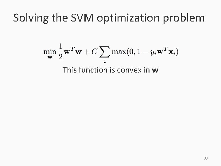
Solving the SVM optimization problem This function is convex in w 30

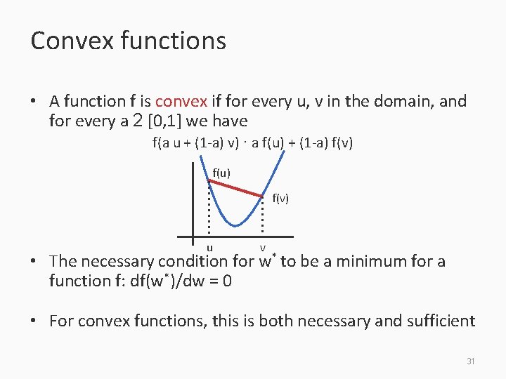
Convex functions • A function f is convex if for every u, v in the domain, and for every a 2 [0, 1] we have f(a u + (1 -a) v) · a f(u) + (1 -a) f(v) f(u) f(v) u v • The necessary condition for w* to be a minimum for a function f: df(w*)/dw = 0 • For convex functions, this is both necessary and sufficient 31

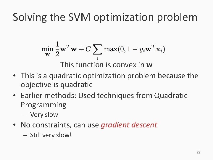
Solving the SVM optimization problem This function is convex in w • This is a quadratic optimization problem because the objective is quadratic • Earlier methods: Used techniques from Quadratic Programming – Very slow • No constraints, can use gradient descent – Still very slow! 32

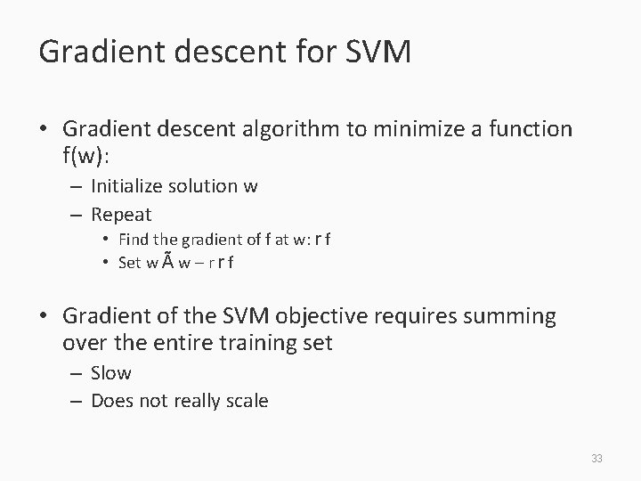
Gradient descent for SVM • Gradient descent algorithm to minimize a function f(w): – Initialize solution w – Repeat • Find the gradient of f at w: r f • Set w à w – r r f • Gradient of the SVM objective requires summing over the entire training set – Slow – Does not really scale 33

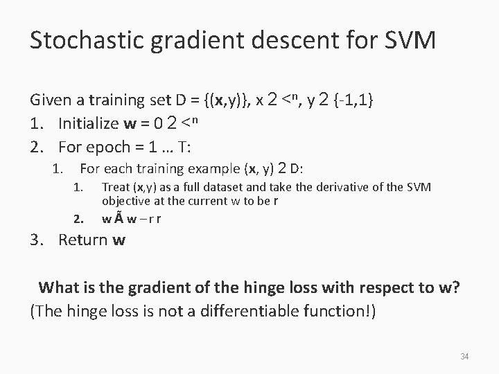
Stochastic gradient descent for SVM Given a training set D = {(x, y)}, x 2 <n, y 2 {-1, 1} 1. Initialize w = 0 2 <n 2. For epoch = 1 … T: 1. For each training example (x, y) 2 D: 1. 2. Treat (x, y) as a full dataset and take the derivative of the SVM objective at the current w to be r wÃw–rr 3. Return w What is the gradient of the hinge loss with respect to w? (The hinge loss is not a differentiable function!) 34

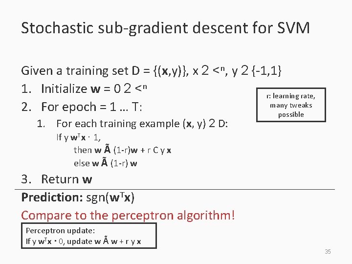
Stochastic sub-gradient descent for SVM Given a training set D = {(x, y)}, x 2 <n, y 2 {-1, 1} 1. Initialize w = 0 2 <n r: learning rate, many tweaks 2. For epoch = 1 … T: possible 1. For each training example (x, y) 2 D: If y w. Tx · 1, then w à (1 -r)w + r C y x else w à (1 -r) w 3. Return w Prediction: sgn(w. Tx) Compare to the perceptron algorithm! Perceptron update: If y w. Tx · 0, update w à w + r y x 35

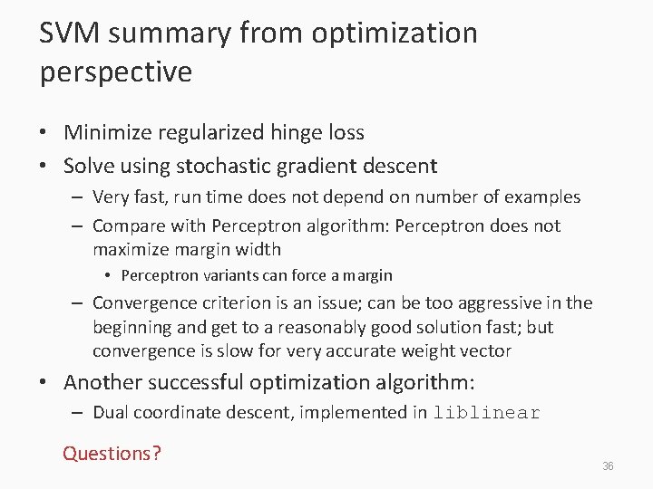
SVM summary from optimization perspective • Minimize regularized hinge loss • Solve using stochastic gradient descent – Very fast, run time does not depend on number of examples – Compare with Perceptron algorithm: Perceptron does not maximize margin width • Perceptron variants can force a margin – Convergence criterion is an issue; can be too aggressive in the beginning and get to a reasonably good solution fast; but convergence is slow for very accurate weight vector • Another successful optimization algorithm: – Dual coordinate descent, implemented in liblinear Questions? 36

Where are we? 1. 2. 3. 4. 5. 6. Supervised learning: The general setting Linear classifiers The Perceptron algorithm Support vector machine Learning as optimization Logistic Regression 37

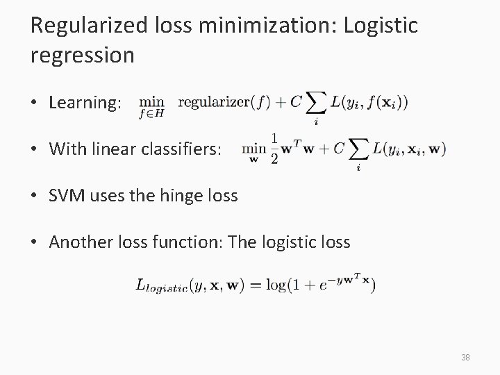
Regularized loss minimization: Logistic regression • Learning: • With linear classifiers: • SVM uses the hinge loss • Another loss function: The logistic loss 38

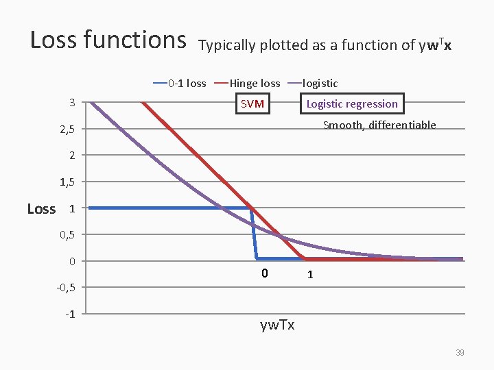
Loss functions Typically plotted as a function of yw. Tx 0 -1 loss 3 Hinge loss SVM logistic Logistic regression Smooth, differentiable 2, 5 2 1, 5 Loss 1 0, 5 0 -0, 5 -1 0 1 yw. Tx 39

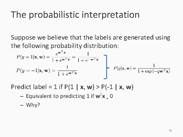
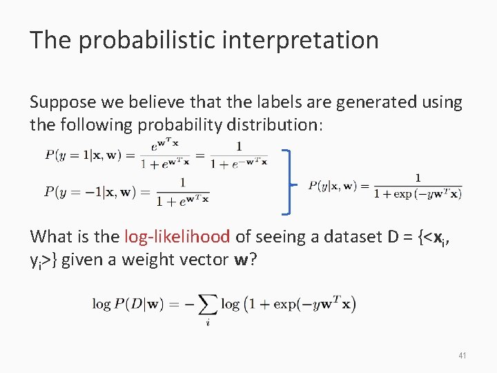
The probabilistic interpretation Suppose we believe that the labels are generated using the following probability distribution: Predict label = 1 if P(1 | x, w) > P(-1 | x, w) – Equivalent to predicting 1 if w. Tx ¸ 0 – Why? 40

The probabilistic interpretation Suppose we believe that the labels are generated using the following probability distribution: What is the log-likelihood of seeing a dataset D = {<xi, yi>} given a weight vector w? 41

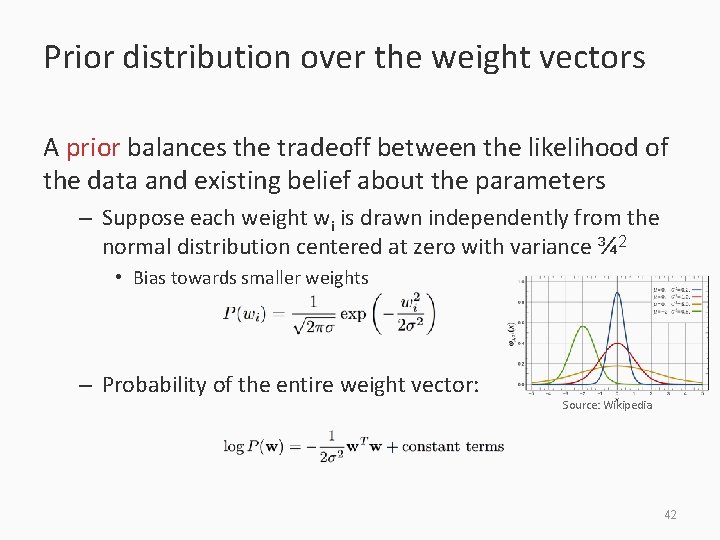
Prior distribution over the weight vectors A prior balances the tradeoff between the likelihood of the data and existing belief about the parameters – Suppose each weight wi is drawn independently from the normal distribution centered at zero with variance ¾ 2 • Bias towards smaller weights – Probability of the entire weight vector: Source: Wikipedia 42

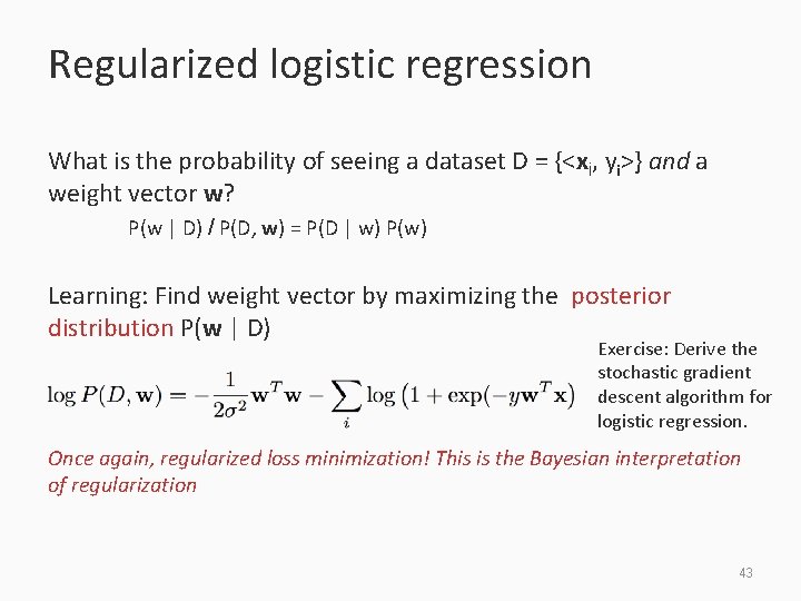
Regularized logistic regression What is the probability of seeing a dataset D = {<xi, yi>} and a weight vector w? P(w | D) / P(D, w) = P(D | w) P(w) Learning: Find weight vector by maximizing the posterior distribution P(w | D) Exercise: Derive the stochastic gradient descent algorithm for logistic regression. Once again, regularized loss minimization! This is the Bayesian interpretation of regularization 43

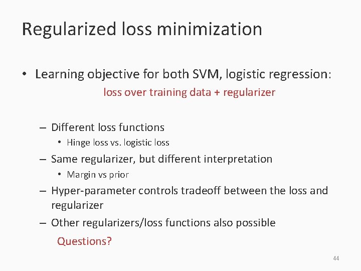
Regularized loss minimization • Learning objective for both SVM, logistic regression: loss over training data + regularizer – Different loss functions • Hinge loss vs. logistic loss – Same regularizer, but different interpretation • Margin vs prior – Hyper-parameter controls tradeoff between the loss and regularizer – Other regularizers/loss functions also possible Questions? 44

Review of binary classification 1. 2. 3. 4. 5. 6. Supervised learning: The general setting Linear classifiers The Perceptron algorithm Support vector machine Learning as optimization Logistic Regression Questions? 45