CIS 700 004 Lecture 4 M Deep vs

CIS 700 -004: Lecture 4 M Deep vs. shallow learning 02/04/19

Course Announcements ● Homework has not been released yet. Keep relaxing : )

Design in deep learning ● Deep learning is not a science yet. ● We don’t know what networks will work for what problems. ● People in general just tweak what worked best. ● We don’t have answers (yet). ● Today, we’ll talk about the start of a science for deep learning - intuition and theory.

The intuitive benefits of depth

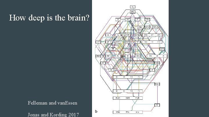
How deep is the brain? Felleman and van. Essen Jonas and Kording 2017

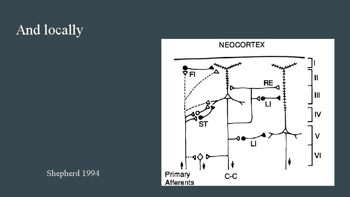
And locally Shepherd 1994

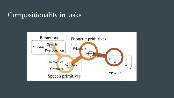
Compositionality in tasks

Expressivity

Expressivity ● We know even shallow neural nets (=1 hidden layer) are universal approximators under various assumptions. ● That could require huge width. ● Given a particular architecture, we can looks at its expressivity, or the set of functions it can approximate. ● Why do we need to look at approximation here?

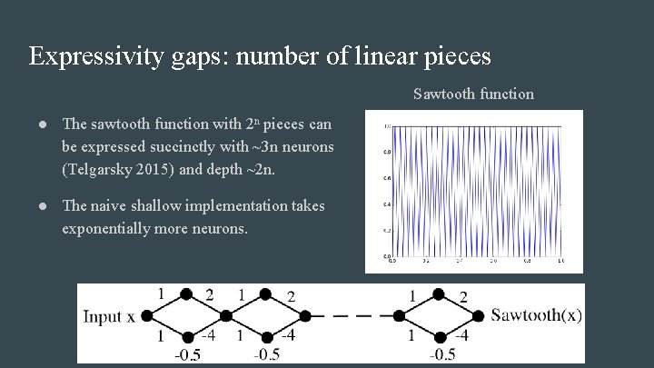
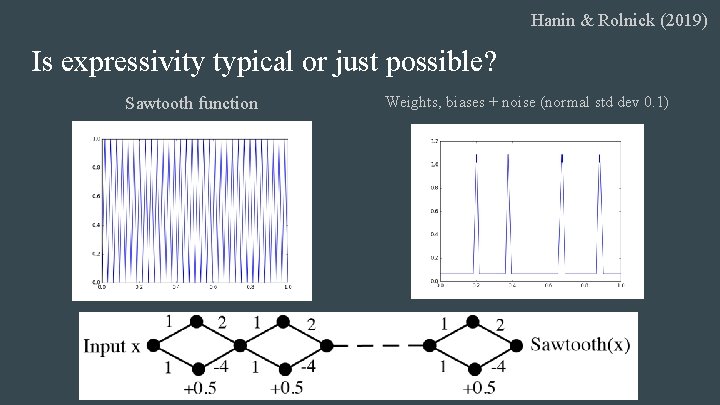
Expressivity gaps: number of linear pieces Sawtooth function ● The sawtooth function with 2 n pieces can be expressed succinctly with ~3 n neurons (Telgarsky 2015) and depth ~2 n. ● The naive shallow implementation takes exponentially more neurons.

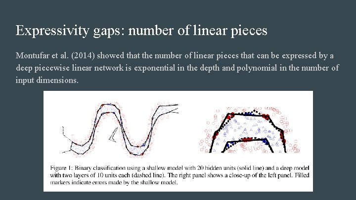
Expressivity gaps: number of linear pieces Montufar et al. (2014) showed that the number of linear pieces that can be expressed by a deep piecewise linear network is exponential in the depth and polynomial in the number of input dimensions.

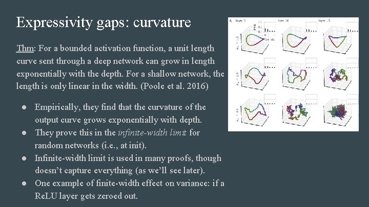
Expressivity gaps: curvature Thm: For a bounded activation function, a unit length curve sent through a deep network can grow in length exponentially with the depth. For a shallow network, the length is only linear in the width. (Poole et al. 2016)

Expressivity gaps: curvature Thm: For a bounded activation function, a unit length curve sent through a deep network can grow in length exponentially with the depth. For a shallow network, the length is only linear in the width. (Poole et al. 2016) ● Empirically, they find that the curvature of the output curve grows exponentially with depth. ● They prove this in the infinite-width limit for random networks (i. e. , at init). ● Infinite-width limit is used in many proofs, though doesn’t capture everything (as we’ll see later). ● One example of finite-width effect on variance: if a Re. LU layer gets zeroed out.

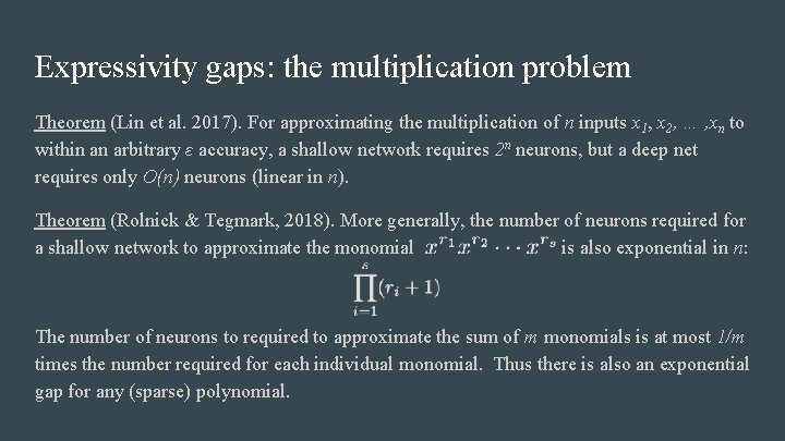
Expressivity gaps: the multiplication problem Theorem (Lin et al. 2017). For approximating the multiplication of n inputs x 1, x 2, … , xn to within an arbitrary ε accuracy, a shallow network requires 2 n neurons, but a deep net requires only O(n) neurons (linear in n). Theorem (Rolnick & Tegmark, 2018). More generally, the number of neurons required for a shallow network to approximate the monomial is also exponential in n: The number of neurons to required to approximate the sum of m monomials is at most 1/m times the number required for each individual monomial. Thus there is also an exponential gap for any (sparse) polynomial.

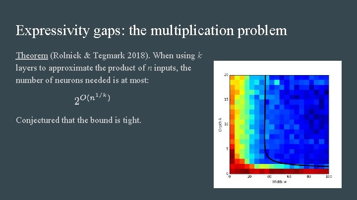
Expressivity gaps: the multiplication problem Theorem (Rolnick & Tegmark 2018). When using k layers to approximate the product of n inputs, the number of neurons needed is at most: Conjectured that the bound is tight.

Learnability

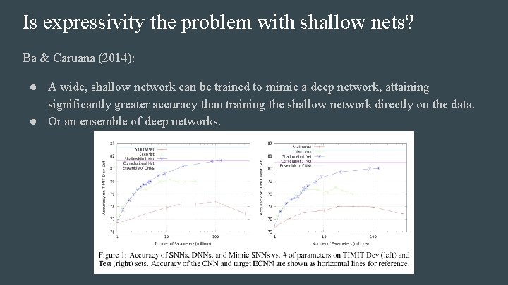
Is expressivity the problem with shallow nets? Ba & Caruana (2014): ● A wide, shallow network can be trained to mimic a deep network, attaining significantly greater accuracy than training the shallow network directly on the data. ● Or an ensemble of deep networks.

Is expressivity the problem with shallow nets? Ba & Caruana (2014): ● A wide, shallow network can be trained to mimic a deep network, attaining significantly greater accuracy than training the shallow network directly on the data. ● Or an ensemble of deep networks. ● The mimic networks output the pre-softmax output of the teach networks. ● Why is there more information here than simply training on the raw data? ● Learnability of deeper networks may be more important than expressivity in practice.

Hanin & Rolnick (2019) Is expressivity typical or just possible? Sawtooth function Weights, biases + noise (normal std dev 0. 1)

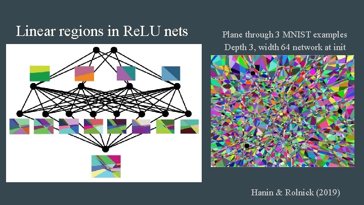
Linear regions in Re. LU nets Plane through 3 MNIST examples Depth 3, width 64 network at init Hanin & Rolnick (2019)

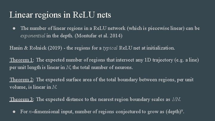
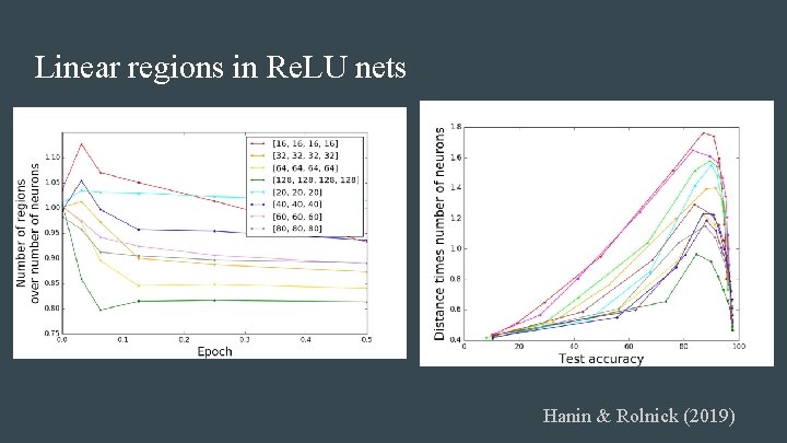
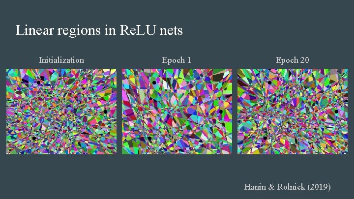
Linear regions in Re. LU nets ● The number of linear regions in a Re. LU network (which is piecewise linear) can be exponential in the depth. (Montufar et al. 2014) Hanin & Rolnick (2019) - the regions for a typical Re. LU net at initialization. Theorem 1: The expected number of regions that intersect any 1 D trajectory (e. g. a line) per unit length is linear in N, the total number of neurons. Theorem 2: The expected surface area of the total boundary between regions, per unit volume, is linear in N. Theorem 3: The expected distance to the nearest region boundary scales as 1/N. ● For n-dimensional input, number of regions conjectured to grow as (depth)n.

Linear regions in Re. LU nets Hanin & Rolnick (2019)

Linear regions in Re. LU nets Initialization Epoch 1 Epoch 20 Hanin & Rolnick (2019)

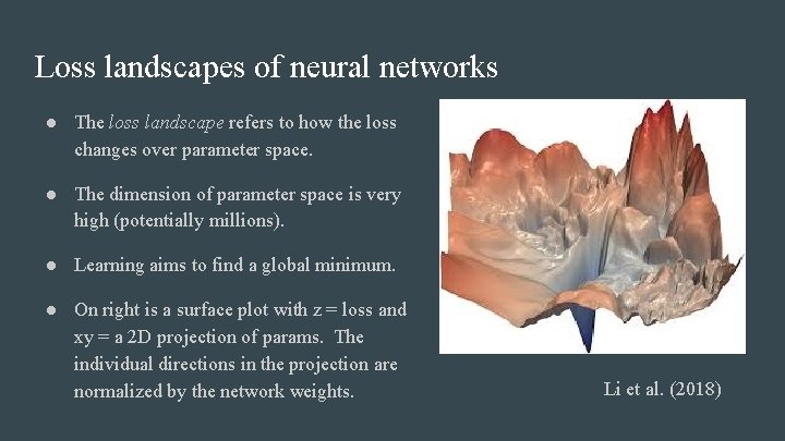
Loss landscapes of neural networks ● The loss landscape refers to how the loss changes over parameter space. ● The dimension of parameter space is very high (potentially millions). ● Learning aims to find a global minimum. ● On right is a surface plot with z = loss and xy = a 2 D projection of params. The individual directions in the projection are normalized by the network weights. Li et al. (2018)

Local optima, saddle points ● The classic worry of optimization is that one can fall into a local optimum. ● (This is why convex optimization is great - local minima are global. ) ● But actually for deep networks there is another problem. ● Local minima are rare but saddle points are common (Dauphin et al. 2014). ● Why is the case? ● Eigenvalues of the Hessian are like for a random matrix, but shifted right by an amount determined by the loss at the point in question (Bray and Dean 2007). ● Saddle points look like plateaus.

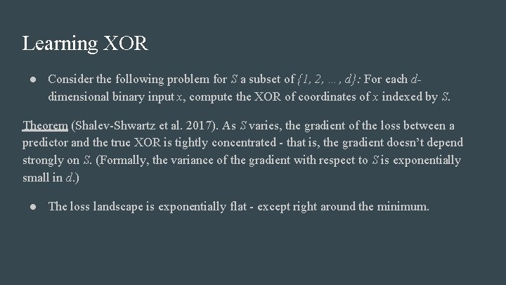
Learning XOR ● Consider the following problem for S a subset of {1, 2, …, d}: For each ddimensional binary input x, compute the XOR of coordinates of x indexed by S. Theorem (Shalev-Shwartz et al. 2017). As S varies, the gradient of the loss between a predictor and the true XOR is tightly concentrated - that is, the gradient doesn’t depend strongly on S. (Formally, the variance of the gradient with respect to S is exponentially small in d. ) ● The loss landscape is exponentially flat - except right around the minimum.

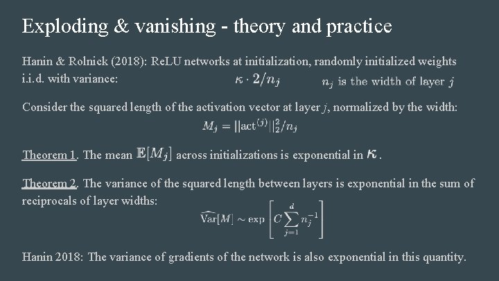
Exploding & vanishing - theory and practice Hanin & Rolnick (2018): Re. LU networks at initialization, randomly initialized weights i. i. d. with variance: Consider the squared length of the activation vector at layer j, normalized by the width: Theorem 1. The mean across initializations is exponential in . Theorem 2. The variance of the squared length between layers is exponential in the sum of reciprocals of layer widths: Hanin 2018: The variance of gradients of the network is also exponential in this quantity.

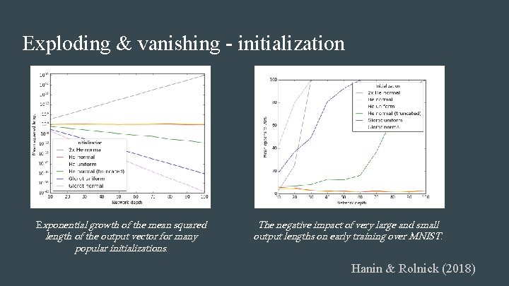
Exploding & vanishing - initialization Exponential growth of the mean squared length of the output vector for many popular initializations. The negative impact of very large and small output lengths on early training over MNIST. Hanin & Rolnick (2018)

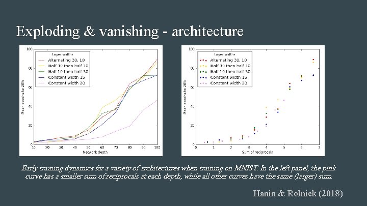
Exploding & vanishing - architecture Early training dynamics for a variety of architectures when training on MNIST. In the left panel, the pink curve has a smaller sum of reciprocals at each depth, while all other curves have the same (larger) sum. Hanin & Rolnick (2018)

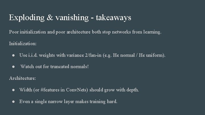
Exploding & vanishing - takeaways Poor initialization and poor architecture both stop networks from learning. Initialization: ● Use i. i. d. weights with variance 2/fan-in (e. g. He normal / He uniform). ● Watch out for truncated normals! Architecture: ● Width (or #features in Conv. Nets) should grow with depth. ● Even a single narrow layer makes training hard.

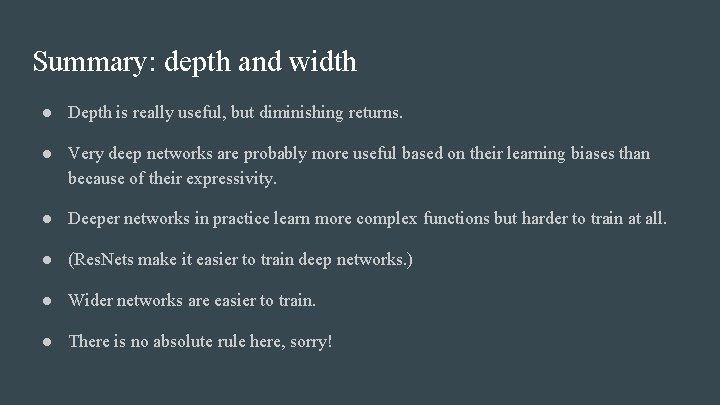
Summary: depth and width ● Depth is really useful, but diminishing returns. ● Very deep networks are probably more useful based on their learning biases than because of their expressivity. ● Deeper networks in practice learn more complex functions but harder to train at all. ● (Res. Nets make it easier to train deep networks. ) ● Wider networks are easier to train. ● There is no absolute rule here, sorry!