CIS 5590 Advanced Topics in LargeScale Machine Learning

CIS 5590: Advanced Topics in Large-Scale Machine Learning Week II: Kernels, Dimension Reduction, and Graphs Instructor: Kai Zhang CIS @ Temple University, Spring 2018

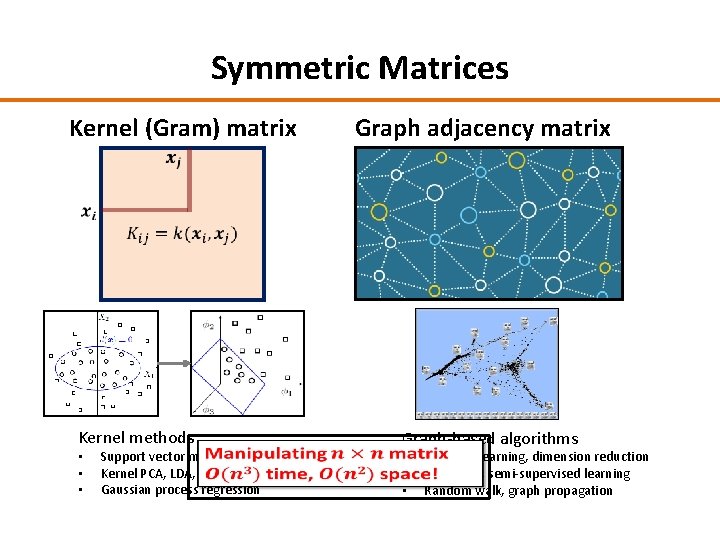
Symmetric Matrices Kernel (Gram) matrix Graph adjacency matrix Kernel methods • • • Support vector machines Kernel PCA, LDA, CCA Gaussian process regression Graph-based algorithms • • • Manifold learning, dimension reduction Clustering, semi-supervised learning Random walk, graph propagation

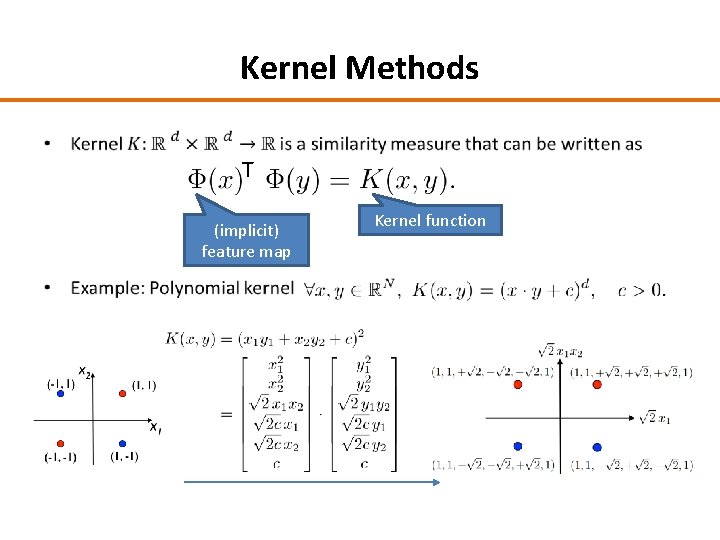
Kernel Methods • T (implicit) feature map Kernel function

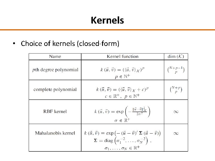
Kernels • Choice of kernels (closed-form)

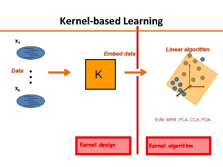
Kernel-based Learning x 1 Embed data Data Linear algorithm K xn SVM, MPM, PCA, CCA, FDA… Kernel design Kernel algorithm

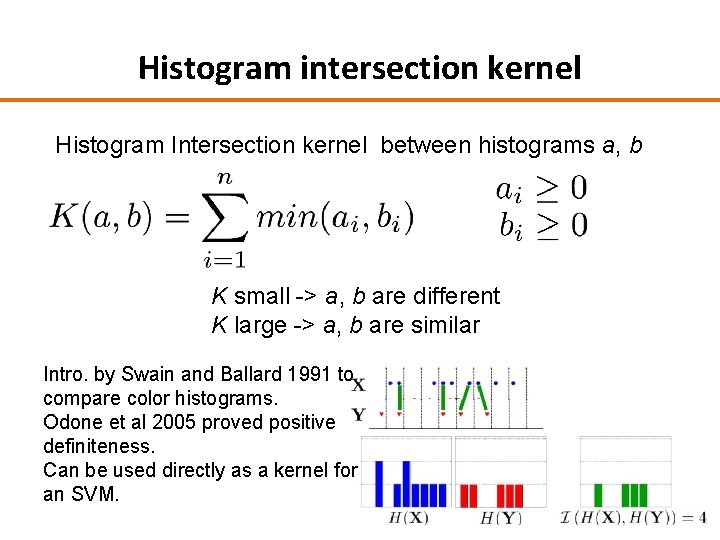
Histogram intersection kernel Histogram Intersection kernel between histograms a, b K small -> a, b are different K large -> a, b are similar Intro. by Swain and Ballard 1991 to compare color histograms. Odone et al 2005 proved positive definiteness. Can be used directly as a kernel for an SVM.

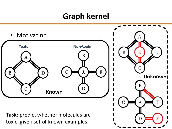
Graph kernel • Motivation A Toxic Non-toxic A B C D C B B Known A D C E Unknown B D C Task: predict whether molecules are toxic, given set of known examples E A E D F

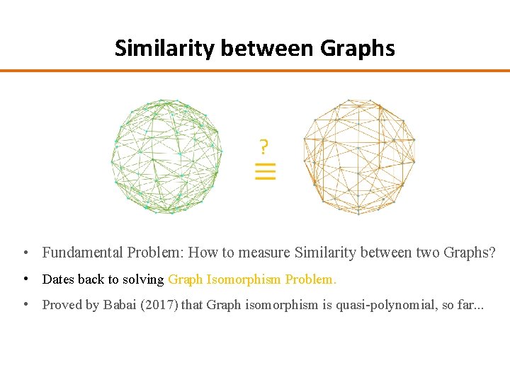
Similarity between Graphs ? • Fundamental Problem: How to measure Similarity between two Graphs? • Dates back to solving Graph Isomorphism Problem. • Proved by Babai (2017) that Graph isomorphism is quasi-polynomial, so far. . .

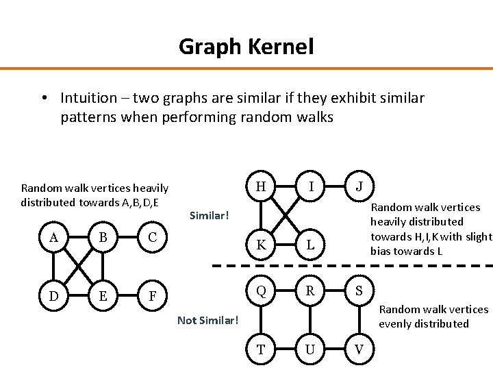
Graph Kernel • Intuition – two graphs are similar if they exhibit similar patterns when performing random walks Random walk vertices heavily distributed towards A, B, D, E A B C D E F H I J Random walk vertices heavily distributed towards H, I, K with slight bias towards L Similar! K L Q R S Random walk vertices evenly distributed Not Similar! T U V

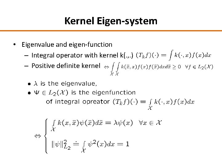
Kernel Eigen-system • Eigenvalue and eigen-function – Integral operator with kernel k(. , . ) – Positive definite kernel

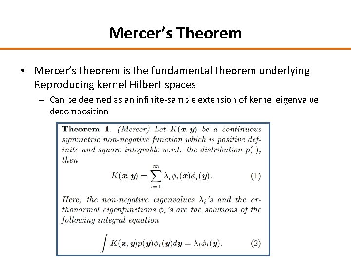
Mercer’s Theorem • Mercer’s theorem is the fundamental theorem underlying Reproducing kernel Hilbert spaces – Can be deemed as an infinite-sample extension of kernel eigenvalue decomposition

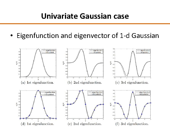
Univariate Gaussian case • Eigenfunction and eigenvector of 1 -d Gaussian

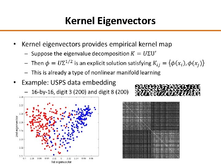
Kernel Eigenvectors •

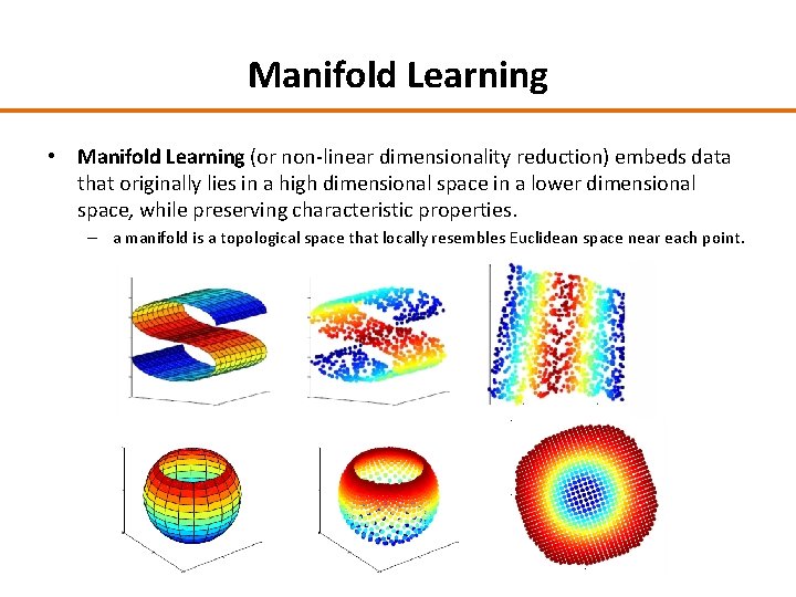
Manifold Learning • Manifold Learning (or non-linear dimensionality reduction) embeds data that originally lies in a high dimensional space in a lower dimensional space, while preserving characteristic properties. – a manifold is a topological space that locally resembles Euclidean space near each point.

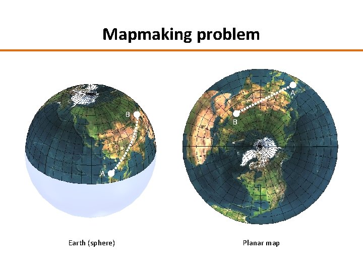
Mapmaking problem A B B A Earth (sphere) Planar map

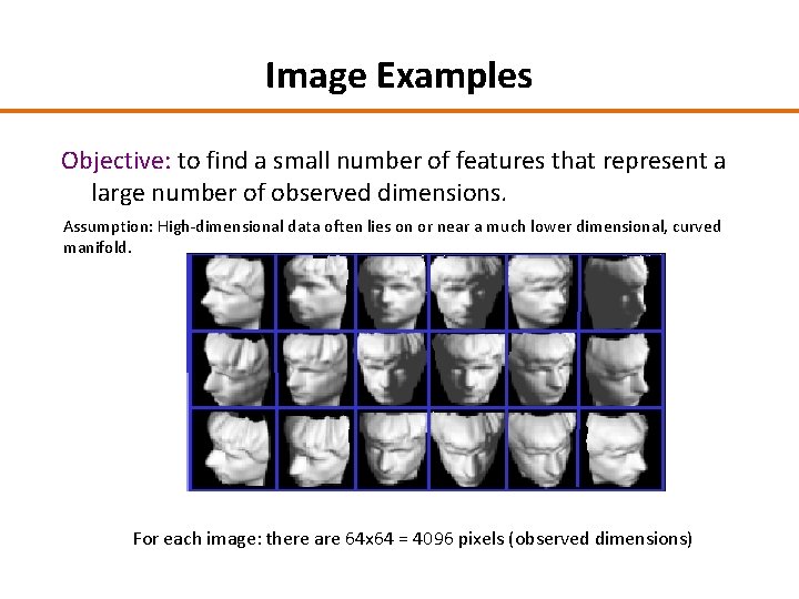
Image Examples Objective: to find a small number of features that represent a large number of observed dimensions. Assumption: High-dimensional data often lies on or near a much lower dimensional, curved manifold. For each image: there are 64 x 64 = 4096 pixels (observed dimensions)

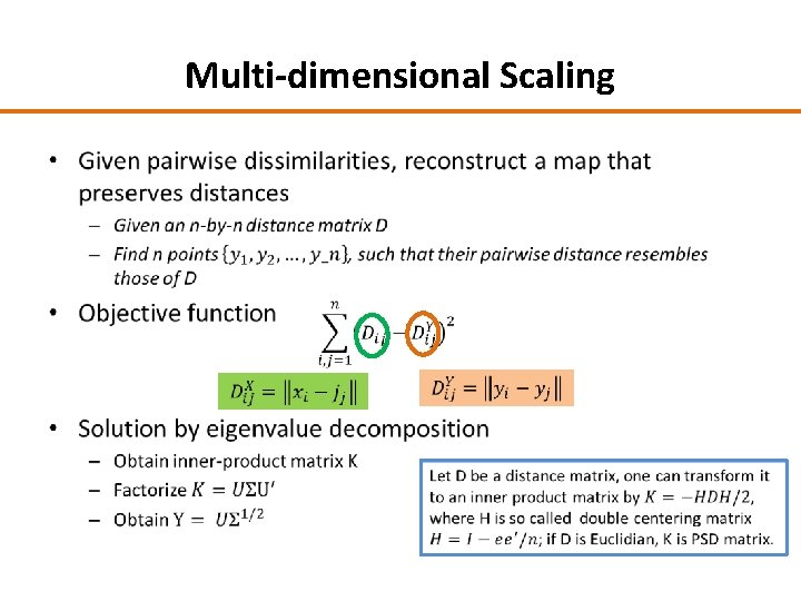
Multi-dimensional Scaling •

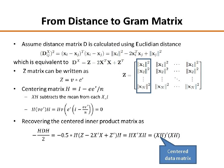
From Distance to Gram Matrix • Centered data matrix

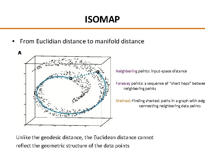
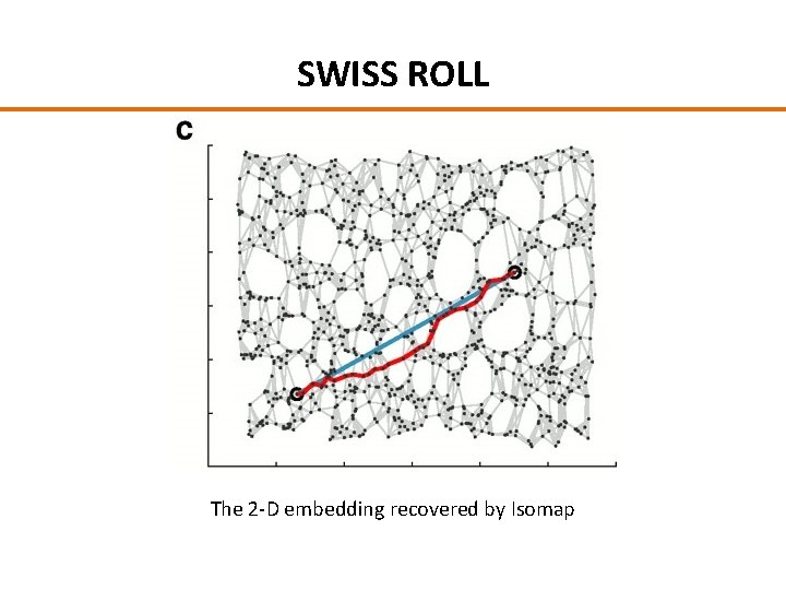
ISOMAP • From Euclidian distance to manifold distance Neighboring points: input-space distance Faraway points: a sequence of “short hops” betwee neighboring points Method: Finding shortest paths in a graph with edge connecting neighboring data points Unlike the geodesic distance, the Euclidean distance cannot reflect the geometric structure of the data points

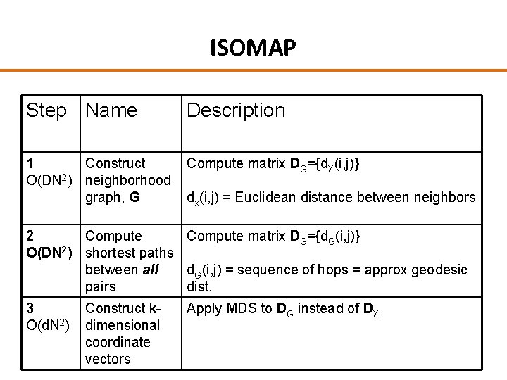
ISOMAP Step Name Description 1 Construct Compute matrix DG={d. X(i, j)} O(DN 2) neighborhood graph, G dx(i, j) = Euclidean distance between neighbors 2 Compute matrix DG={d. G(i, j)} O(DN 2) shortest paths between all d. G(i, j) = sequence of hops = approx geodesic pairs dist. 3 O(d. N 2) Construct kdimensional coordinate vectors Apply MDS to DG instead of DX

SWISS ROLL The 2 -D embedding recovered by Isomap

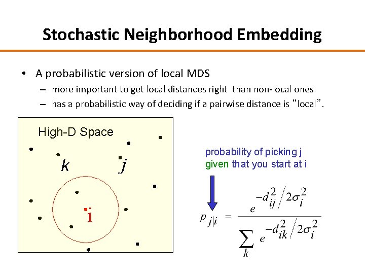
Stochastic Neighborhood Embedding • A probabilistic version of local MDS – more important to get local distances right than non-local ones – has a probabilistic way of deciding if a pairwise distance is “local”. High-D Space j k i probability of picking j given that you start at i

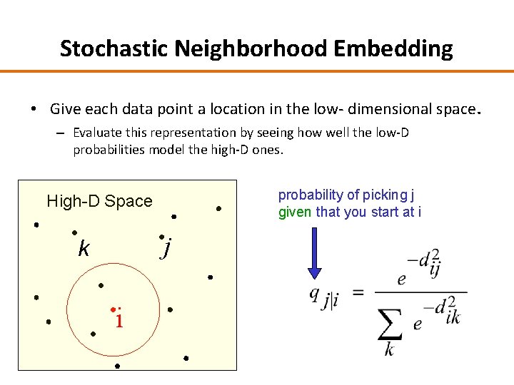
Stochastic Neighborhood Embedding • Give each data point a location in the low- dimensional space. – Evaluate this representation by seeing how well the low-D probabilities model the high-D ones. probability of picking j given that you start at i High-D Space j k i

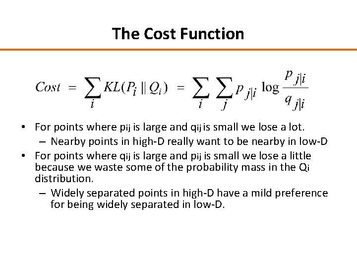
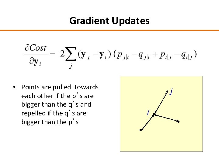
The Cost Function • For points where pij is large and qij is small we lose a lot. – Nearby points in high-D really want to be nearby in low-D • For points where qij is large and pij is small we lose a little because we waste some of the probability mass in the Qi distribution. – Widely separated points in high-D have a mild preference for being widely separated in low-D.

Gradient Updates • Points are pulled towards each other if the p’s are bigger than the q’s and repelled if the q’s are bigger than the p’s j i

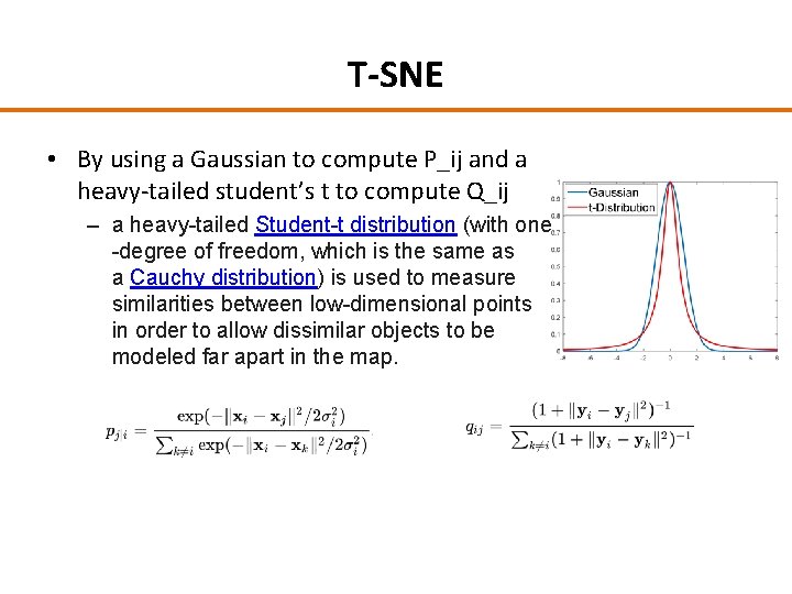
T-SNE • By using a Gaussian to compute P_ij and a heavy-tailed student’s t to compute Q_ij – a heavy-tailed Student-t distribution (with one -degree of freedom, which is the same as a Cauchy distribution) is used to measure similarities between low-dimensional points in order to allow dissimilar objects to be modeled far apart in the map.

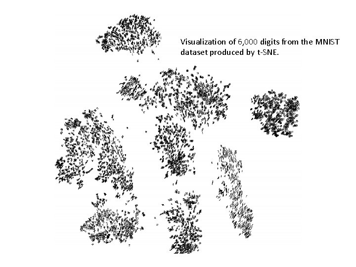
Visualization of 6, 000 digits from the MNIST dataset produced by t-SNE.

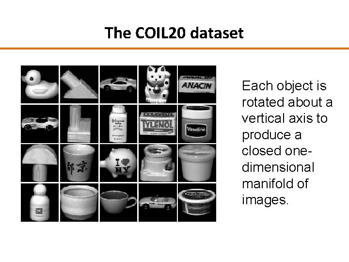
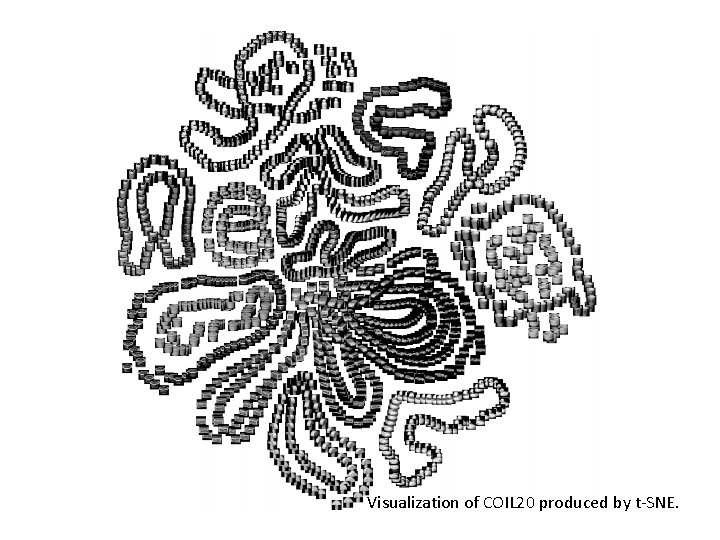
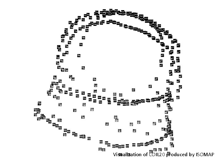
The COIL 20 dataset Each object is rotated about a vertical axis to produce a closed onedimensional manifold of images.

Visualization of COIL 20 produced by t-SNE.

Visualization of COIL 20 produced by ISOMAP

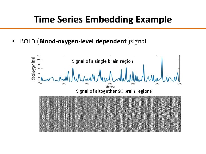
Time Series Embedding Example • BOLD (Blood-oxygen-level dependent )signal Signal of a single brain region Signal of altogether 90 brain regions

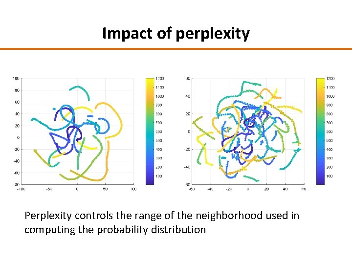
Impact of perplexity Perplexity controls the range of the neighborhood used in computing the probability distribution

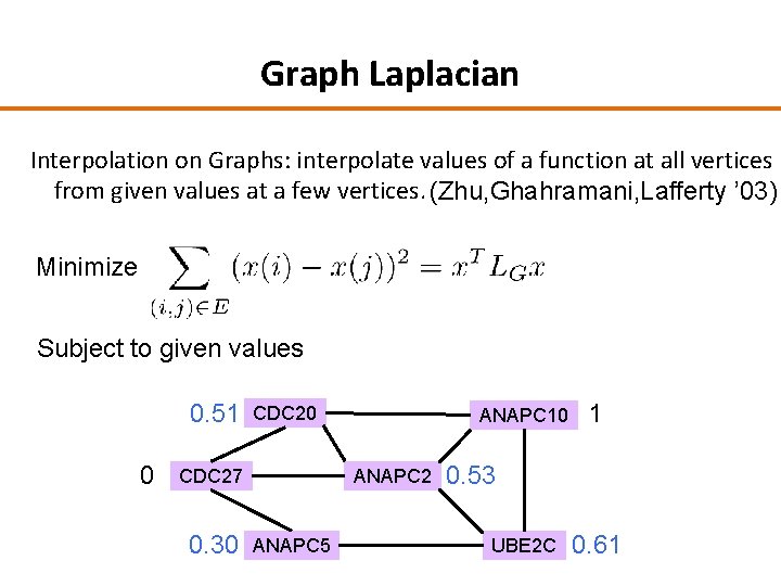
Graph Laplacian Interpolation on Graphs: interpolate values of a function at all vertices from given values at a few vertices. (Zhu, Ghahramani, Lafferty ’ 03) Minimize Subject to given values 0. 51 0 CDC 27 0. 30 ANAPC 10 ANAPC 2 ANAPC 5 1 0. 53 UBE 2 C 0. 61

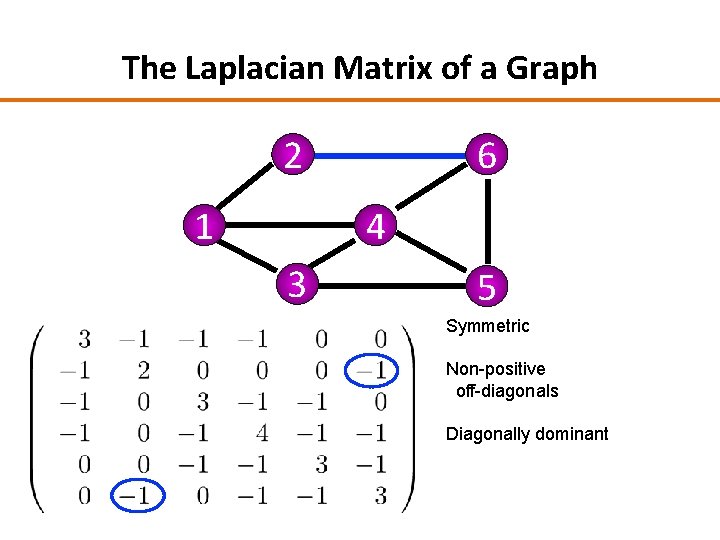
The Laplacian Matrix of a Graph 2 1 6 4 3 5 Symmetric Non-positive off-diagonals Diagonally dominant

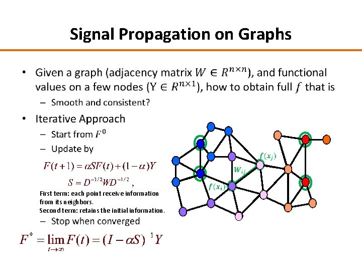
Signal Propagation on Graphs • First term: each point receive information from its neighbors. Second term: retains the initial information. -

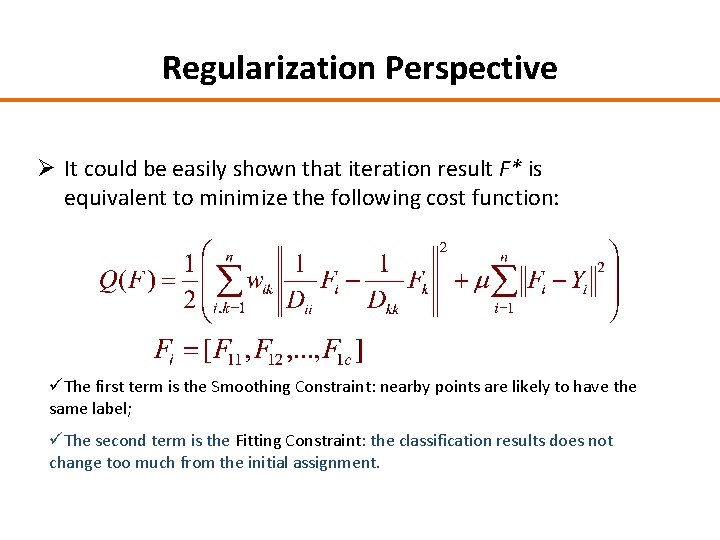
Regularization Perspective Ø It could be easily shown that iteration result F* is equivalent to minimize the following cost function: üThe first term is the Smoothing Constraint: nearby points are likely to have the same label; üThe second term is the Fitting Constraint: the classification results does not change too much from the initial assignment.

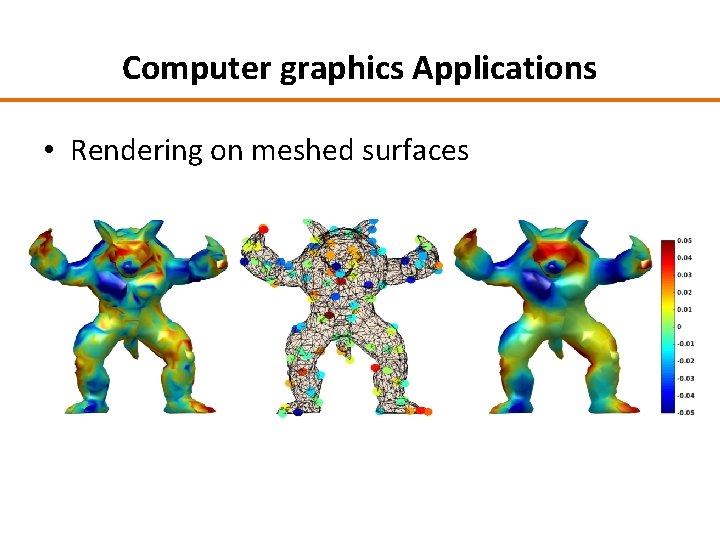
Computer graphics Applications • Rendering on meshed surfaces

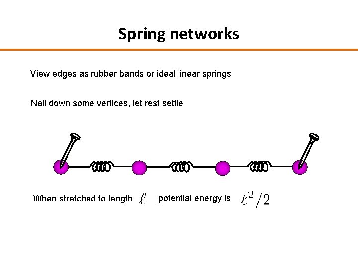
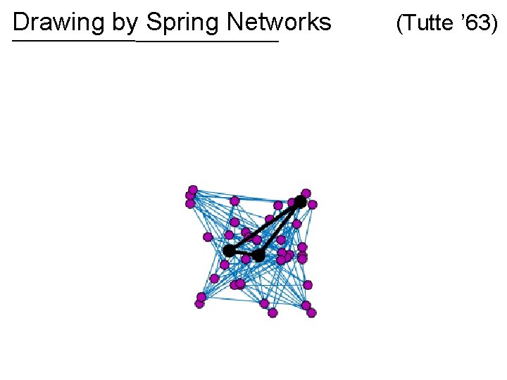
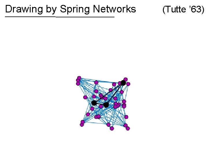
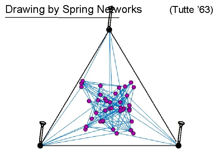
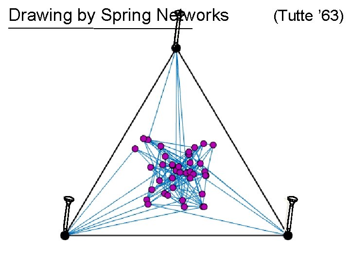
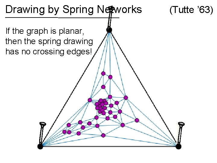
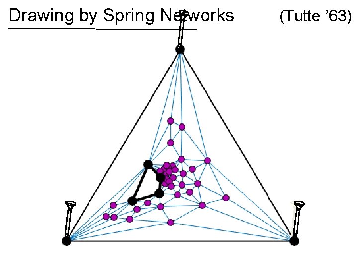
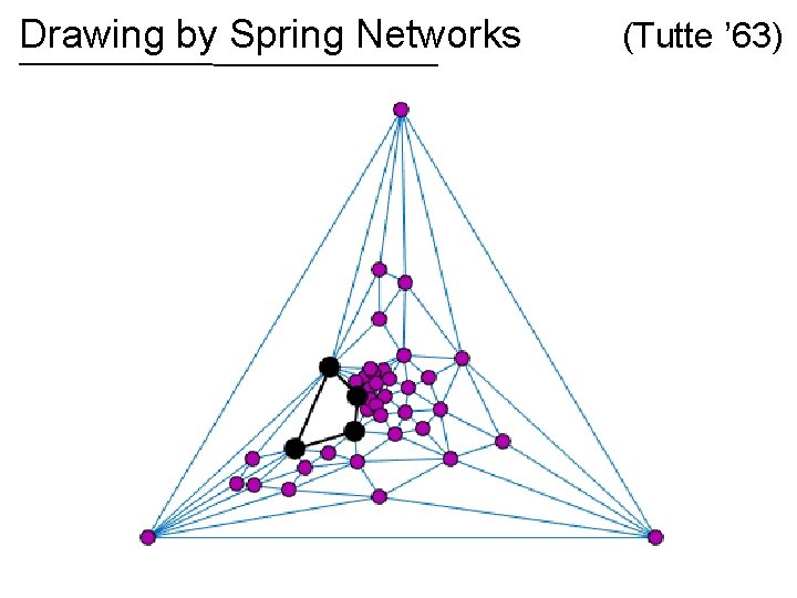
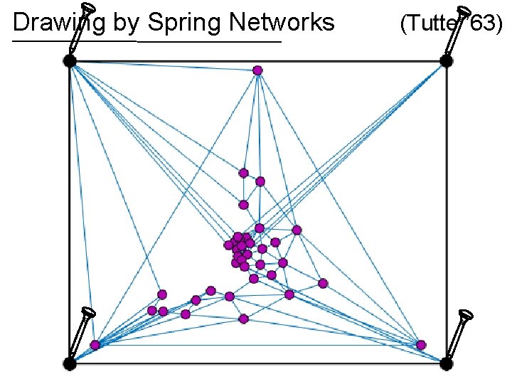
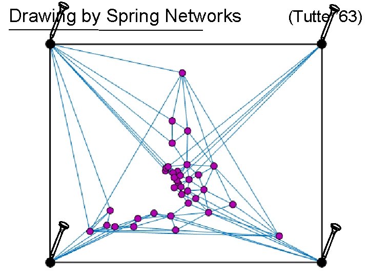
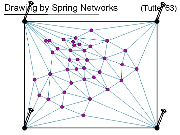
Spring networks View edges as rubber bands or ideal linear springs Nail down some vertices, let rest settle When stretched to length potential energy is

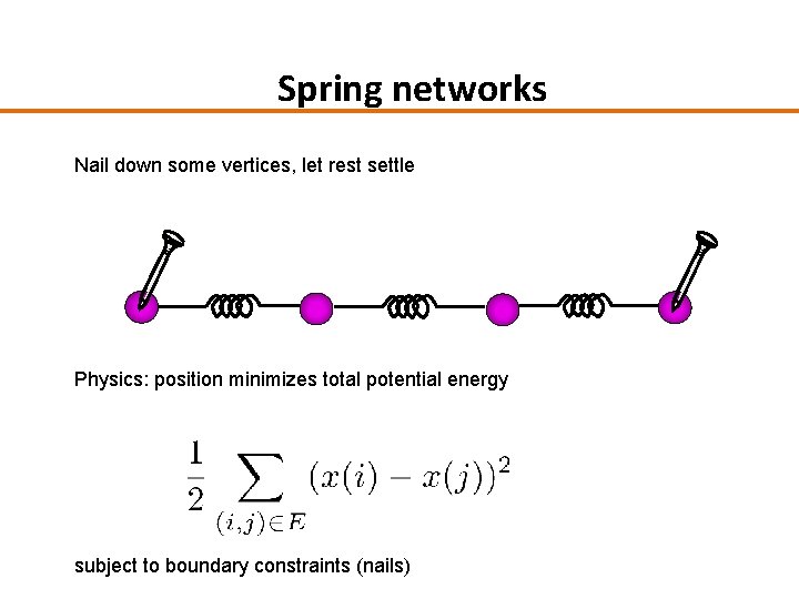
Spring networks Nail down some vertices, let rest settle Physics: position minimizes total potential energy subject to boundary constraints (nails)

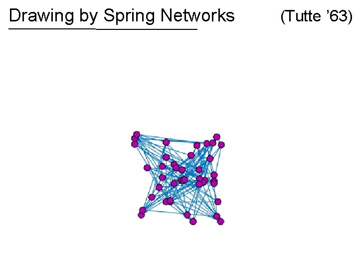
Drawing by Spring Networks (Tutte ’ 63)

Drawing by Spring Networks (Tutte ’ 63)

Drawing by Spring Networks (Tutte ’ 63)

Drawing by Spring Networks (Tutte ’ 63)

Drawing by Spring Networks (Tutte ’ 63)

Drawing by Spring Networks If the graph is planar, then the spring drawing has no crossing edges! (Tutte ’ 63)

Drawing by Spring Networks (Tutte ’ 63)

Drawing by Spring Networks (Tutte ’ 63)

Drawing by Spring Networks (Tutte ’ 63)

Drawing by Spring Networks (Tutte ’ 63)

Drawing by Spring Networks (Tutte ’ 63)

Recent Advances • Auto-encoder – an artificial neural network used for unsupervised learning of efficient codings. The goal is to learn a representation (encoding) for a set of data, typically for the purpose of dimensionality reduction. • Word embedding – a set of language modeling and feature learning techniques in natural language processing (NLP) where words or phrases from the vocabulary are mapped to vectors of real numbers.

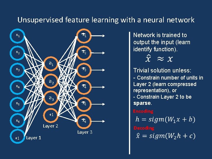
Unsupervised feature learning with a neural network x 1 x 2 a 1 x 3 a 2 x 4 a 3 x 5 +1 x 6 +1 Layer 2 Layer 1 Network is trained to output the input (learn identify function). x 3 Trivial solution unless: - Constrain number of units in x 4 Layer 2 (learn compressed representation), or - Constrain Layer 2 to be sparse. x 5 Encoding x 6 Layer 3 Decoding

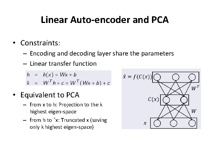
Linear Auto-encoder and PCA • Constraints: – Encoding and decoding layer share the parameters – Linear transfer function • Equivalent to PCA – from x to h: Projection to the k highest eigen-space – from h to ˆx: Truncated x (saving only k highest eigen-space)

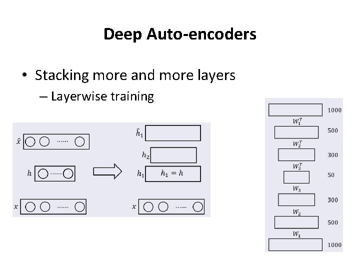
Deep Auto-encoders • Stacking more and more layers – Layerwise training

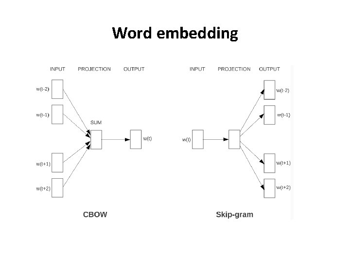
Word embedding • Goal: Associate a low-dimensional, dense vector w with each word w ∈ V so that similar words (in a distributional sense) share a similar vector representation. You shall know a word by the company it keeps. (J. R. Firth, 1957) • Implications – A word ought to be able to predict its context (word 2 vec Skip-Gram) – A context ought to be able to predict its missing word (word 2 vec CBOW) Tomas Mikolov et al. “Distributed Representations of Words and Phrases and their Compositionality”. In: Advances in Neural Information Processing Systems 26. 2013, pp. 3111– 3119

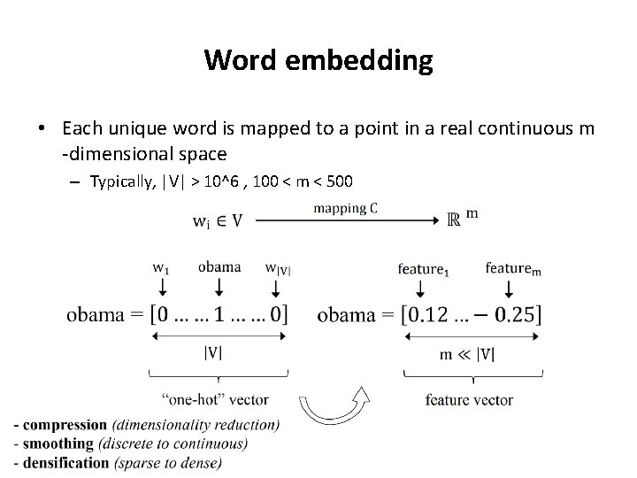
Word embedding • Each unique word is mapped to a point in a real continuous m -dimensional space – Typically, |V| > 10^6 , 100 < m < 500

Word embedding

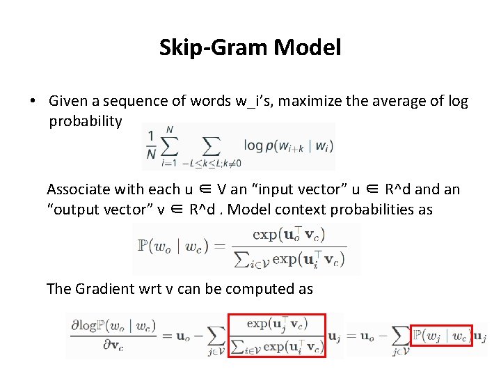
Skip-Gram Model • Given a sequence of words w_i’s, maximize the average of log probability Associate with each u ∈ V an “input vector” u ∈ R^d an “output vector” v ∈ R^d. Model context probabilities as The Gradient wrt v can be computed as

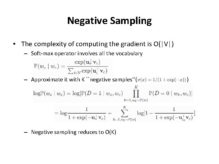
Negative Sampling • The complexity of computing the gradient is O(|V|) – Soft-max operator involves all the vocabulary – Approximate it with K ``negative samples’’( ) – Negative sampling reduces to O(K)