CHME 420 Mass Transfer 5 Mass Transfer Equipment

CHME 420: Mass Transfer 5. Mass Transfer Equipment 5 b. Modeling of Continuous Contact Mass Transfer Equipment and Absorption/Stripping Processes

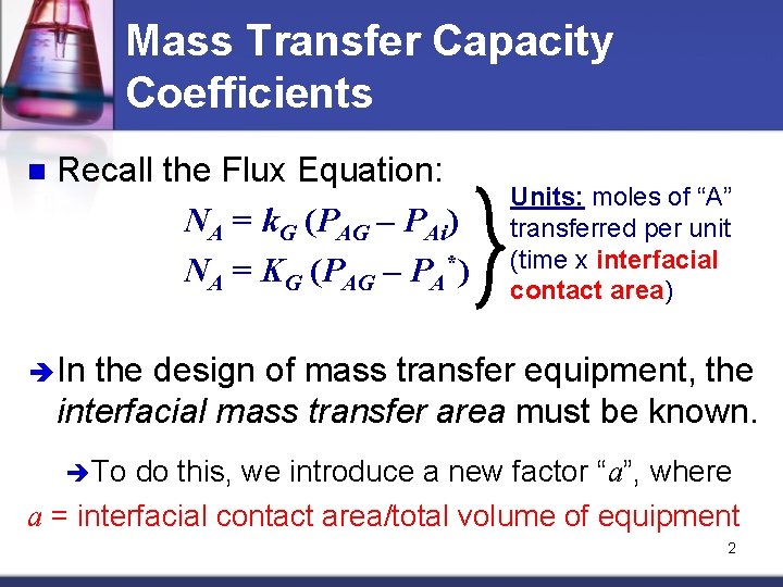
Mass Transfer Capacity Coefficients n Recall the Flux Equation: NA = k. G (PAG – PAi) NA = KG (PAG – PA*) Units: moles of “A” transferred per unit (time x interfacial contact area) In the design of mass transfer equipment, the interfacial mass transfer area must be known. To do this, we introduce a new factor “a”, where a = interfacial contact area/total volume of equipment 2

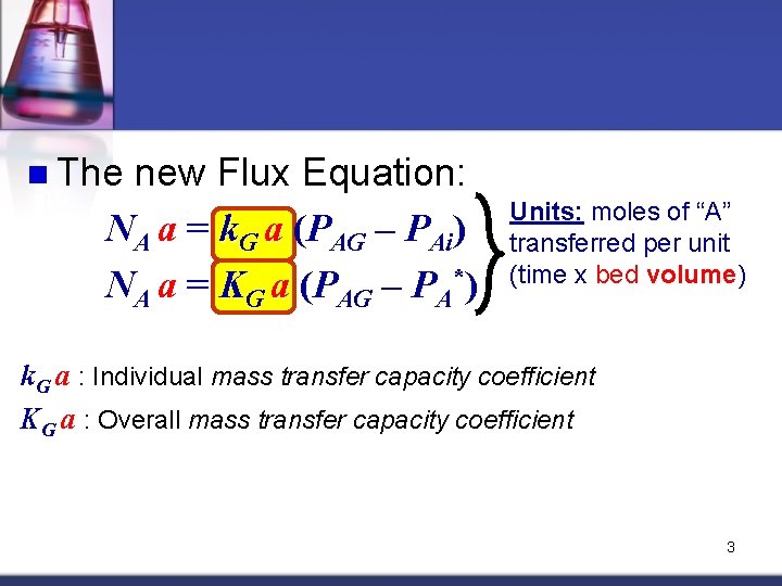
n The new Flux Equation: NA a = k. G a (PAG – PAi) NA a = KG a (PAG – PA*) Units: moles of “A” transferred per unit (time x bed volume) k. G a : Individual mass transfer capacity coefficient KG a : Overall mass transfer capacity coefficient 3

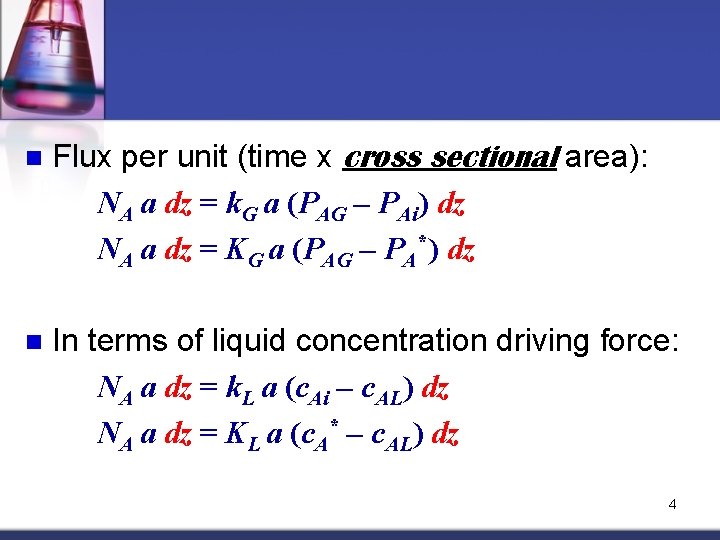
n Flux per unit (time x cross sectional area): NA a dz = k. G a (PAG – PAi) dz NA a dz = KG a (PAG – PA*) dz n In terms of liquid concentration driving force: NA a dz = k. L a (c. Ai – c. AL) dz NA a dz = KL a (c. A* – c. AL) dz 4

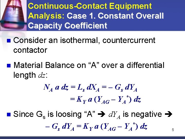
Continuous-Contact Equipment Analysis: Case 1. Constant Overall Capacity Coefficient n Consider an isothermal, countercurrent contactor n Material Balance on “A” over a differential length dz: NA a dz = Ls d. XA = – Gs d. YA = KY a (YAG – YA*) dz n Since Gs is loosing “A” d. YA is negative – Gs d. YA = KY a (YAG – YA*) dz 5

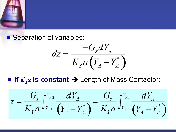
n Separation of variables: n If KYa is constant Length of Mass Contactor: 6

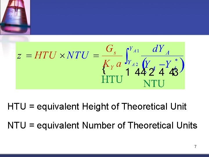
HTU = equivalent Height of Theoretical Unit NTU = equivalent Number of Theoretical Units 7

How to evaluate the integral “NTU”? 1. 2. Draw the equilibrium curve and operating line Start from Y 1 on the operating line: 1. 2. 3. 4. drop a vertical line from that point to the equilibrium line obtain the corresponding Y 1* reading from the equilibrium line Y Y 1 Y *1 Y 2 Repeat the procedure with other Y values until reaching Y 2 * Y 2 Record the values of Y and X 2 the corresponding Y* X 8

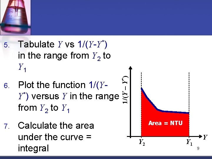
Tabulate Y vs 1/(Y-Y*) in the range from Y 2 to Y 1 6. Plot the function 1/(YY*) versus Y in the range from Y 2 to Y 1 7. Calculate the area under the curve = integral 1/(Y – Y*) 5. Area = NTU Y 2 Y 1 Y 9

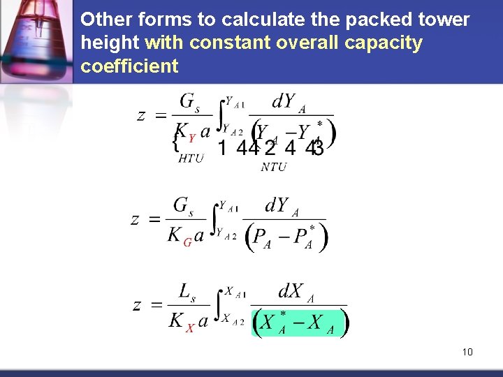
Other forms to calculate the packed tower height with constant overall capacity coefficient 10

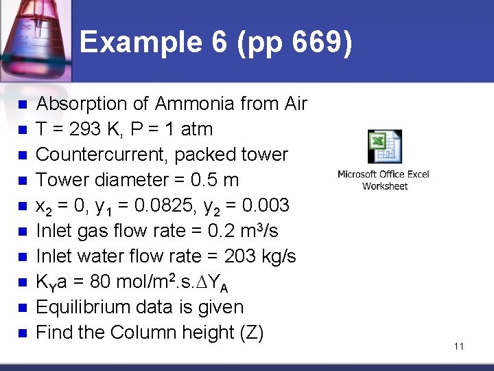
Example 6 (pp 669) n n n n n Absorption of Ammonia from Air T = 293 K, P = 1 atm Countercurrent, packed tower Tower diameter = 0. 5 m x 2 = 0, y 1 = 0. 0825, y 2 = 0. 003 Inlet gas flow rate = 0. 2 m 3/s Inlet water flow rate = 203 kg/s KYa = 80 mol/m 2. s. DYA Equilibrium data is given Find the Column height (Z) 11

Continuous-Contact Equipment Analysis: Case 2. Variable Overall Capacity Coefficient Consider an isothermal, countercurrent contactor n Since K may vary with concentration (unless the equilibrium line is straight) overall capacity coefficients (K a) may also be variable Individual capacity coefficients (k a), which is assumed to be constant at constant T, will be used n 12

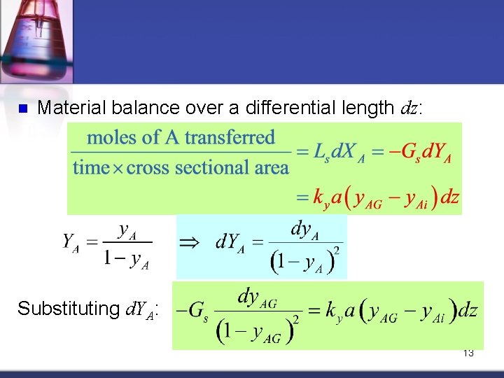
n Material balance over a differential length dz: Substituting d. YA: 13

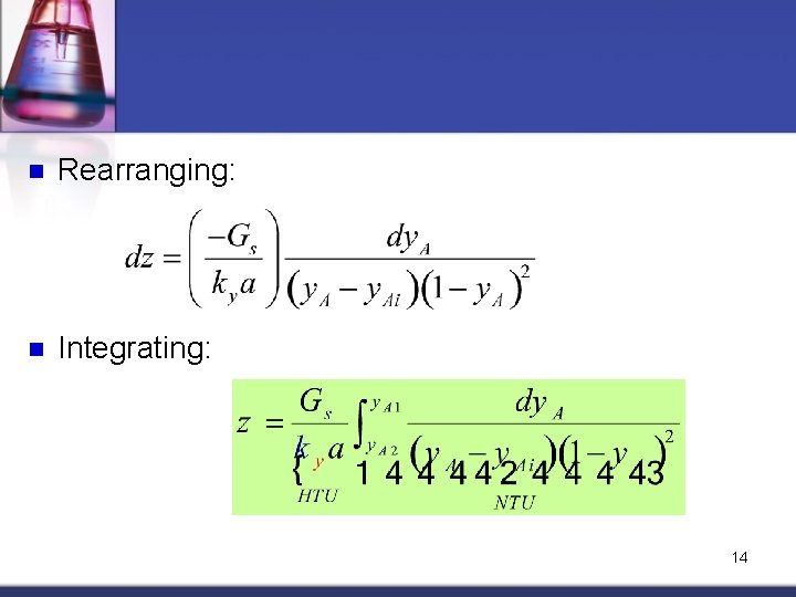
n Rearranging: n Integrating: 14

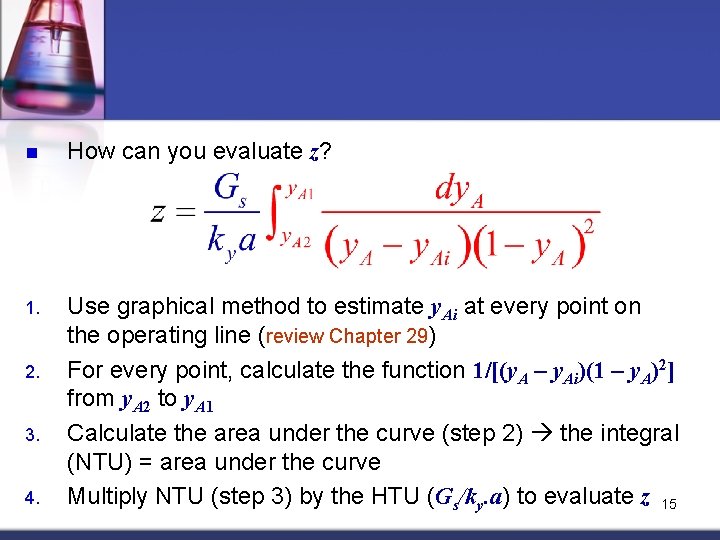
n How can you evaluate z? 1. Use graphical method to estimate y. Ai at every point on the operating line (review Chapter 29) For every point, calculate the function 1/[(y. A – y. Ai)(1 – y. A)2] from y. A 2 to y. A 1 Calculate the area under the curve (step 2) the integral (NTU) = area under the curve Multiply NTU (step 3) by the HTU (Gs/ky. a). a to evaluate z 15 2. 3. 4.

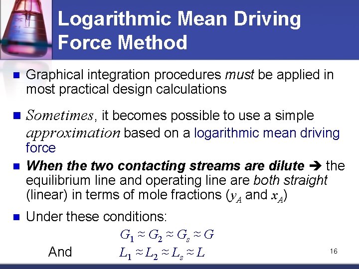
Logarithmic Mean Driving Force Method n Graphical integration procedures must be applied in most practical design calculations n Sometimes, it becomes possible to use a simple approximation based on a logarithmic mean driving n n force When the two contacting streams are dilute the equilibrium line and operating line are both straight (linear) in terms of mole fractions (y. A and x. A) Under these conditions: G 1 ≈ G 2 ≈ Gs ≈ G And L 1 ≈ L 2 ≈ Ls ≈ L 16

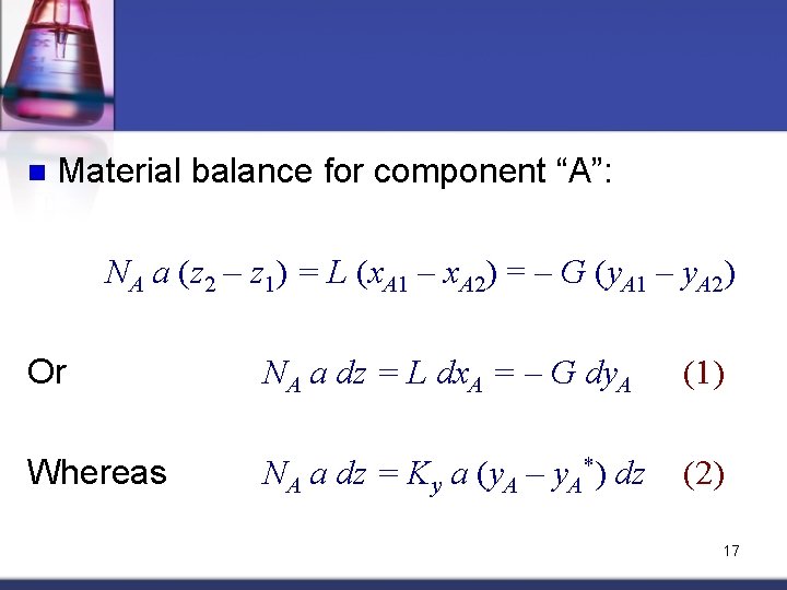
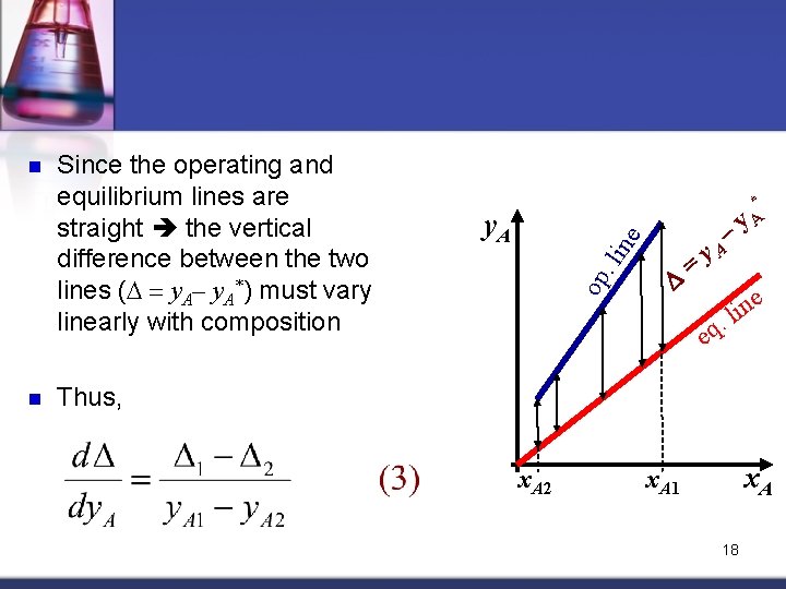
n Material balance for component “A”: NA a (z 2 – z 1) = L (x. A 1 – x. A 2) = – G (y. A 1 – y. A 2) Or NA a dz = L dx. A = – G dy. A (1) Whereas NA a dz = Ky a (y. A – y. A*) dz (2) 17

n Since the operating and equilibrium lines are straight the vertical difference between the two lines (D = y. A– y. A*) must vary linearly with composition y. A op. li ne n – D = * y. A e n i. l q e Thus, x. A 2 x. A 1 18

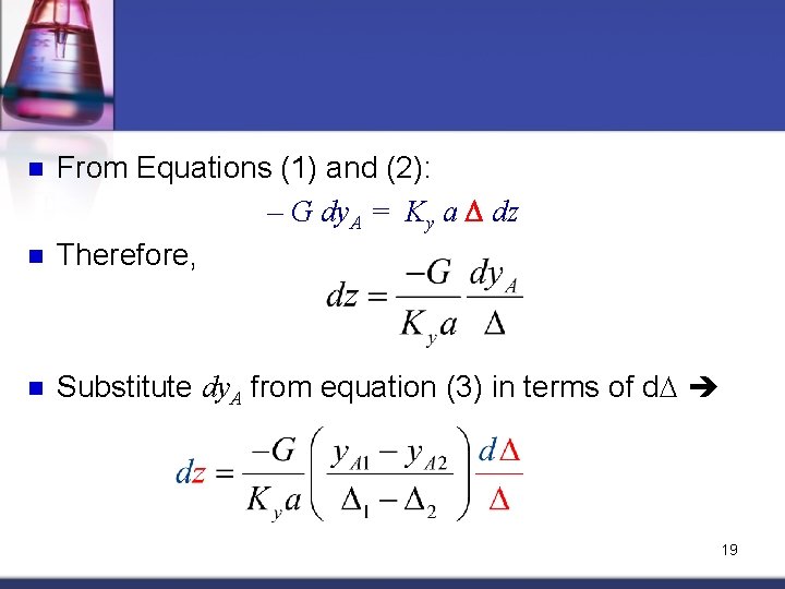
n From Equations (1) and (2): – G dy. A = Ky a D dz Therefore, n Substitute dy. A from equation (3) in terms of d. D n 19

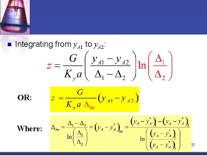
n Integrating from y. A 1 to y. A 2: OR: Where: 20

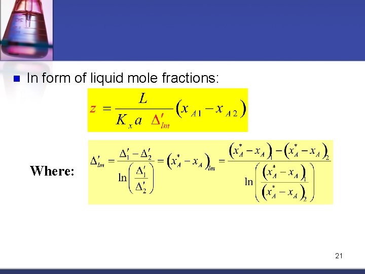
n In form of liquid mole fractions: Where: 21

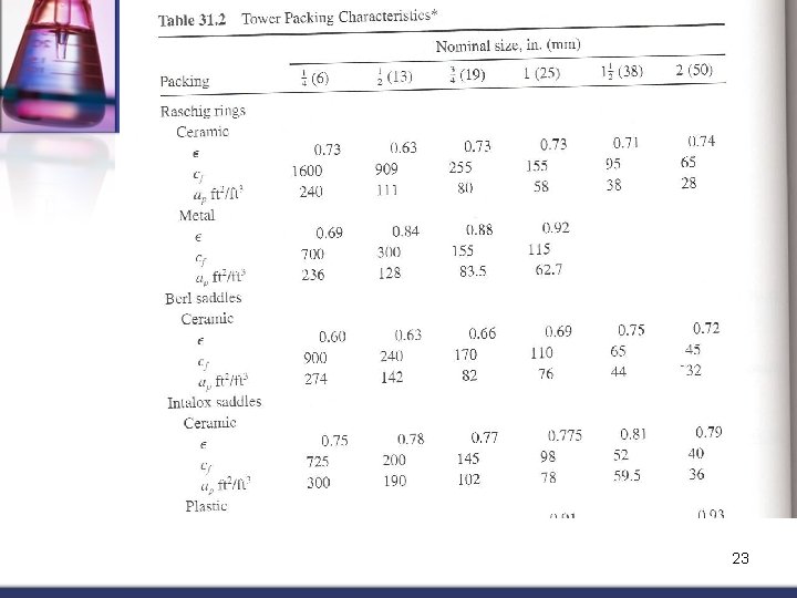
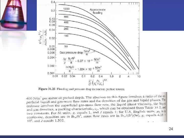
Estimation of Packed Tower Diameter n Various packing types can be used in packed towers. Table 31 -2 lists properties of most common packing materials n Diameter of packed column is established to handle the maximum mass flow rates per unit area of the two phases to be contacted (L’ and G’) n When knowing the pressure drop per meter of packing (Pa/m) and the flow rates of G and L streams we can obtain the cross sectional area of the tower using Figure 31. 25 22

23

24