ChiSquare Goodness of Fit Test In general the

Chi-Square Goodness of Fit Test

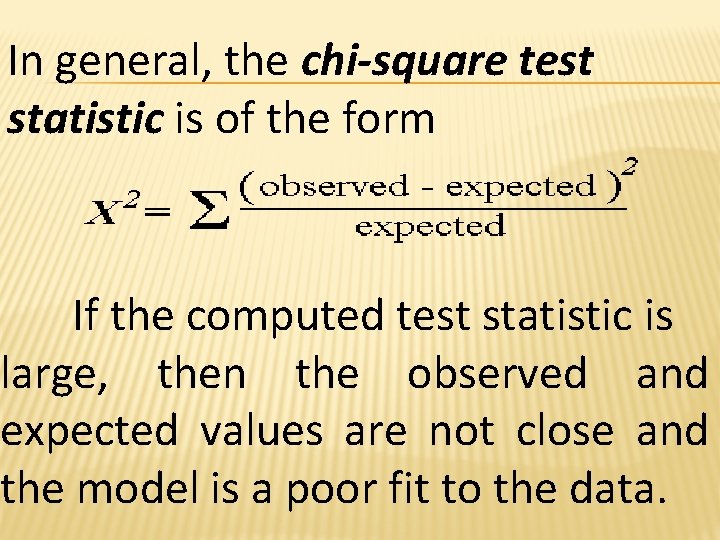
In general, the chi-square test statistic is of the form If the computed test statistic is large, then the observed and expected values are not close and the model is a poor fit to the data.

When to Use the Chi-Square Goodness of Fit Test The chi-square goodness of fit test is appropriate when the following conditions are met: • The sampling method is simple random sampling. • The population is at least 10 times as large as the sample. • The variable under study is categorical. • The expected value of the number of sample observations in each level of the variable is at least 5. This approach consists of four steps: (1) state the hypotheses, (2) formulate an analysis plan, (3) analyze sample data, and (4) interpret

State the Hypotheses Every hypothesis test requires the analyst to state a null hypothesis and an alternative hypothesis. The hypotheses are stated in such a way that they are mutually exclusive. That is, if one is true, the other must be false; and vice versa. For a chi-square goodness of fit test, the hypotheses take the following form. H : The data are consistent with a specified 0 distribution. Ha: The data are not consistent with a specified distribution. Typically, the null hypothesis specifies the proportion of observations at each level of the categorical variable. The alternative hypothesis is that at least one of the specified proportions is not true.

Formulate an Analysis Plan The analysis plan describes how to use sample data to accept or reject the null hypothesis. The plan should specify the following elements. • Significance level. Often, researchers choose significance levels equal to 0. 01 (99% confident), 0. 05 (95% confident) , or 0. 10 (90% confident. • Test method. Use the chi-square goodness of fit test to determine whether observed sample frequencies differ significantly from expected frequencies specified in the null hypothesis. The chi-square goodness of fit test is described in the next section, and demonstrated in the sample problem at the end of this lesson.

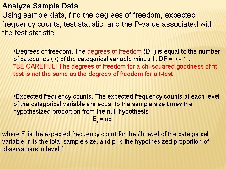
Analyze Sample Data Using sample data, find the degrees of freedom, expected frequency counts, test statistic, and the P-value associated with the test statistic. • Degrees of freedom. The degrees of freedom (DF) is equal to the number of categories (k) of the categorical variable minus 1: DF = k - 1. *BE CAREFUL! The degrees of freedom for a chi-squared goodness of fit test is not the same as the degrees of freedom for a t-test. • Expected frequency counts. The expected frequency counts at each level of the categorical variable are equal to the sample size times the hypothesized proportion from the null hypothesis Ei = npi where Ei is the expected frequency count for the ith level of the categorical variable, n is the total sample size, and pi is the hypothesized proportion of observations in level i.

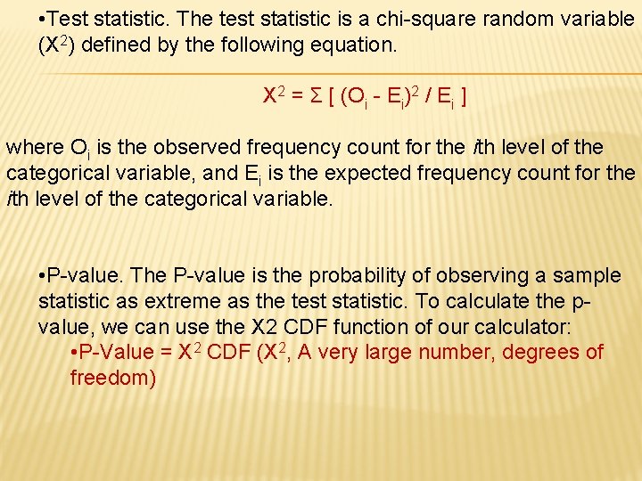
• Test statistic. The test statistic is a chi-square random variable (Χ 2) defined by the following equation. Χ 2 = Σ [ (Oi - Ei)2 / Ei ] where Oi is the observed frequency count for the ith level of the categorical variable, and Ei is the expected frequency count for the ith level of the categorical variable. • P-value. The P-value is the probability of observing a sample statistic as extreme as the test statistic. To calculate the pvalue, we can use the X 2 CDF function of our calculator: • P-Value = X 2 CDF (X 2, A very large number, degrees of freedom)

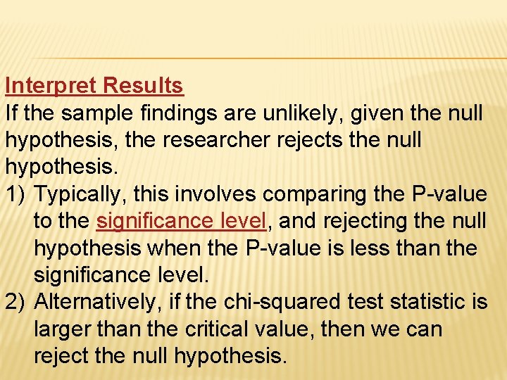
Interpret Results If the sample findings are unlikely, given the null hypothesis, the researcher rejects the null hypothesis. 1) Typically, this involves comparing the P-value to the significance level, and rejecting the null hypothesis when the P-value is less than the significance level. 2) Alternatively, if the chi-squared test statistic is larger than the critical value, then we can reject the null hypothesis.

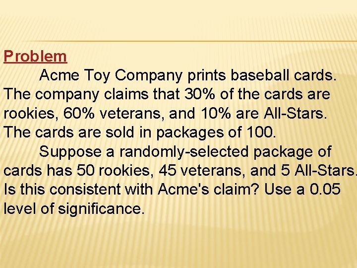
Problem Acme Toy Company prints baseball cards. The company claims that 30% of the cards are rookies, 60% veterans, and 10% are All-Stars. The cards are sold in packages of 100. Suppose a randomly-selected package of cards has 50 rookies, 45 veterans, and 5 All-Stars. Is this consistent with Acme's claim? Use a 0. 05 level of significance.

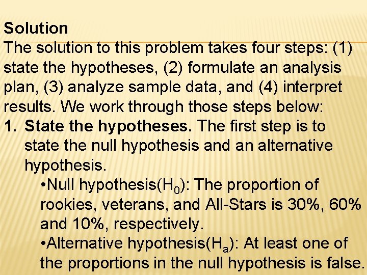
Solution The solution to this problem takes four steps: (1) state the hypotheses, (2) formulate an analysis plan, (3) analyze sample data, and (4) interpret results. We work through those steps below: 1. State the hypotheses. The first step is to state the null hypothesis and an alternative hypothesis. • Null hypothesis(H 0): The proportion of rookies, veterans, and All-Stars is 30%, 60% and 10%, respectively. • Alternative hypothesis(Ha): At least one of the proportions in the null hypothesis is false.

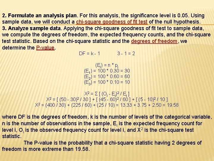
2. Formulate an analysis plan. For this analysis, the significance level is 0. 05. Using sample data, we will conduct a chi-square goodness of fit test of the null hypothesis. 3. Analyze sample data. Applying the chi-square goodness of fit test to sample data, we compute the degrees of freedom, the expected frequency counts, and the chi-square test statistic. Based on the chi-square statistic and the degrees of freedom, we determine the P-value. DF = k - 1 3 -1=2 (Ei) = n * pi (E 1) = 100 * 0. 30 = 30 (E 2) = 100 * 0. 60 = 60 (E 3) = 100 * 0. 10 = 10 Χ 2 = Σ [ (Oi - Ei)2 / Ei ] Χ 2 = [ (50 - 30)2 / 30 ] + [ (45 - 60)2 / 60 ] + [ (5 - 10)2 / 10 ] Χ 2 = (400 / 30) + (225 / 60) + (25 / 10) = 13. 33 + 3. 75 + 2. 50 = 19. 58 where DF is the degrees of freedom, k is the number of levels of the categorical variable, n is the number of observations in the sample, Ei is the expected frequency count for level i, Oi is the observed frequency count for level i, and Χ 2 is the chi-square test statistic. The P-value is the probability that a chi-square statistic having 2 degrees of freedom is more extreme than 19. 58.

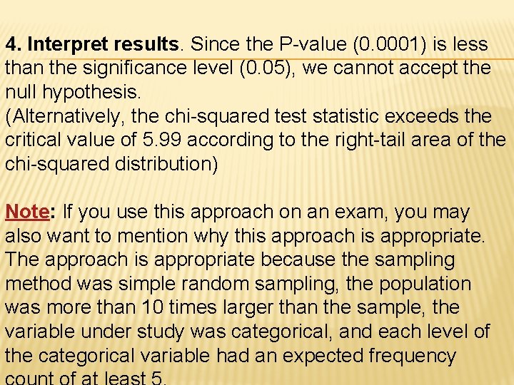
4. Interpret results. Since the P-value (0. 0001) is less than the significance level (0. 05), we cannot accept the null hypothesis. (Alternatively, the chi-squared test statistic exceeds the critical value of 5. 99 according to the right-tail area of the chi-squared distribution) Note: If you use this approach on an exam, you may also want to mention why this approach is appropriate. The approach is appropriate because the sampling method was simple random sampling, the population was more than 10 times larger than the sample, the variable under study was categorical, and each level of the categorical variable had an expected frequency

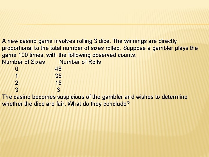
A new casino game involves rolling 3 dice. The winnings are directly proportional to the total number of sixes rolled. Suppose a gambler plays the game 100 times, with the following observed counts: Number of Sixes Number of Rolls 0 48 1 35 2 15 3 3 The casino becomes suspicious of the gambler and wishes to determine whether the dice are fair. What do they conclude?