CHI SQUARE USES OF CHI SQUARE Chi Square

CHI SQUARE

USES OF CHI SQUARE Chi Square is the most common and simple non-parametric test of significance investigating associations between categories of nominal variables where observations can be classified into discrete categories and treated as frequencies.

CHI SQUARE For Example: Is there a significant preference for one of three brands of toothpaste among a sample of chnildren; Is there a significant association between membership or not of a trade union among fulltime and part-time employees; Are there gender preferences for various types of investment category Interval data can be degraded to nominal to enable use of chi square, e. g. age into age groups, income into income groups.

USE OF CHI SQUARE • Chi Square tests hypotheses about the independence (or association) of frequency counts in various categories. The hypotheses are: • H 0 where the variables are statistically independent or no statistical association, and • H 1 where the variables are statistically dependent or associated. • For example H 0 would state that there is no significant association between your gender and which toothpaste you prefer; or that union membership is independent of (not associated with) type of employment, i. e. that the cross-categories from each variable are independent of each other.

TWO FORMS OF CHI SQUARE • • • There are two forms 1. Goodness-of-Fit Chi Square 2. Cross-tabulations (contingency tables) But to whichever of these uses chi square is put, the general principle remains the same. We compare the observed proportions in a sample with the expected proportions and apply the chi-square test to determine whether the difference between observed and expected proportions is likely to be a function of sampling error (non-significant - retaining the null hypothesis H 0 ) or unlikely to be a function of sampling error (significant association - reject the null hypothesis and support alternate hypothesis - H 1 ).

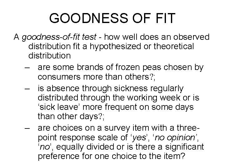
GOODNESS OF FIT A goodness-of-fit test - how well does an observed distribution fit a hypothesized or theoretical distribution – are some brands of frozen peas chosen by consumers more than others ; – is absence through sickness regularly distributed through the working week or is ‘sick leave’ more frequent on some days than other days ; – are choices on a survey item with a threepoint response scale of ‘yes’, ‘no opinion’, ‘no’, equally divided or is there a significant preference for one choice to the item?

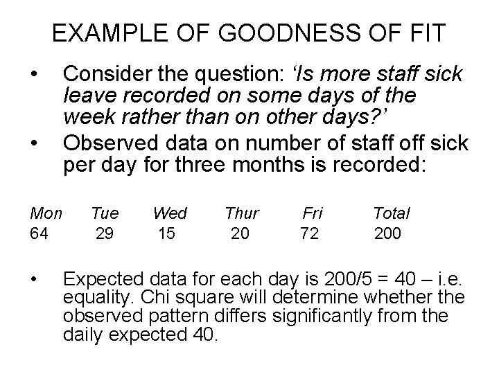
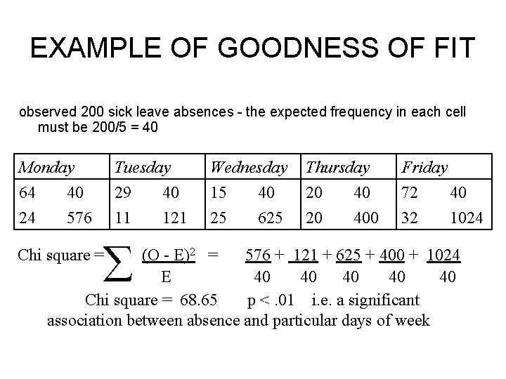
EXAMPLE OF GOODNESS OF FIT • • Mon 64 • Consider the question: ‘Is more staff sick leave recorded on some days of the week rather than on other days? ’ Observed data on number of staff off sick per day for three months is recorded: Tue 29 Wed 15 Thur 20 Fri 72 Total 200 Expected data for each day is 200/5 = 40 – i. e. equality. Chi square will determine whether the observed pattern differs significantly from the daily expected 40.

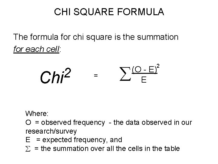
CHI SQUARE FORMULA The formula for chi square is the summation for each cell: 2 Chi = 2 (O - E) E Where: O = observed frequency - the data observed in our research/survey E = expected frequency, and = the summation over all the cells in the table

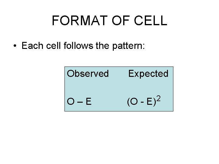
FORMAT OF CELL • Each cell follows the pattern: Observed Expected O–E (O - E) 2

EXAMPLE OF GOODNESS OF FIT observed 200 sick leave absences - the expected frequency in each cell must be 200/5 = 40 Monday 64 40 24 576 Tuesday 29 40 11 121 Chi square = Wednesday 15 40 25 625 Thursday 20 400 Friday 72 40 32 1024 (O - E)2 = 576 + 121 + 625 + 400 + 1024 E 40 40 40 Chi square = 68. 65 p <. 01 i. e. a significant association between absence and particular days of week

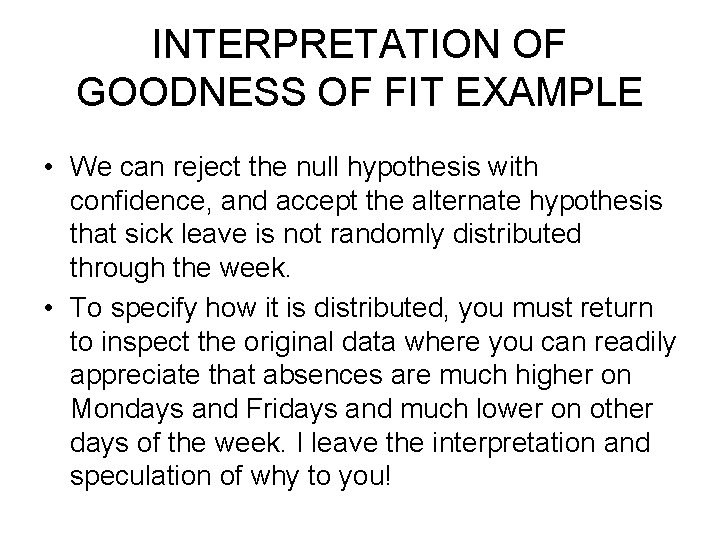
INTERPRETATION OF GOODNESS OF FIT EXAMPLE • We can reject the null hypothesis with confidence, and accept the alternate hypothesis that sick leave is not randomly distributed through the week. • To specify how it is distributed, you must return to inspect the original data where you can readily appreciate that absences are much higher on Mondays and Fridays and much lower on other days of the week. I leave the interpretation and speculation of why to you!

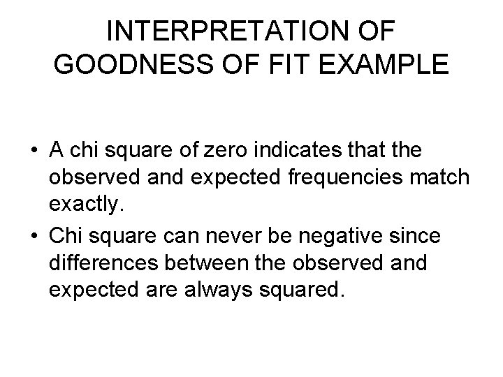
INTERPRETATION OF GOODNESS OF FIT EXAMPLE • A chi square of zero indicates that the observed and expected frequencies match exactly. • Chi square can never be negative since differences between the observed and expected are always squared.

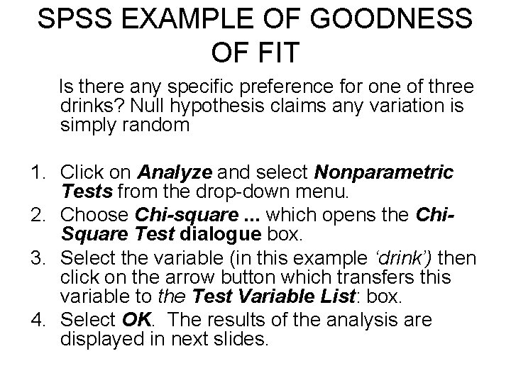
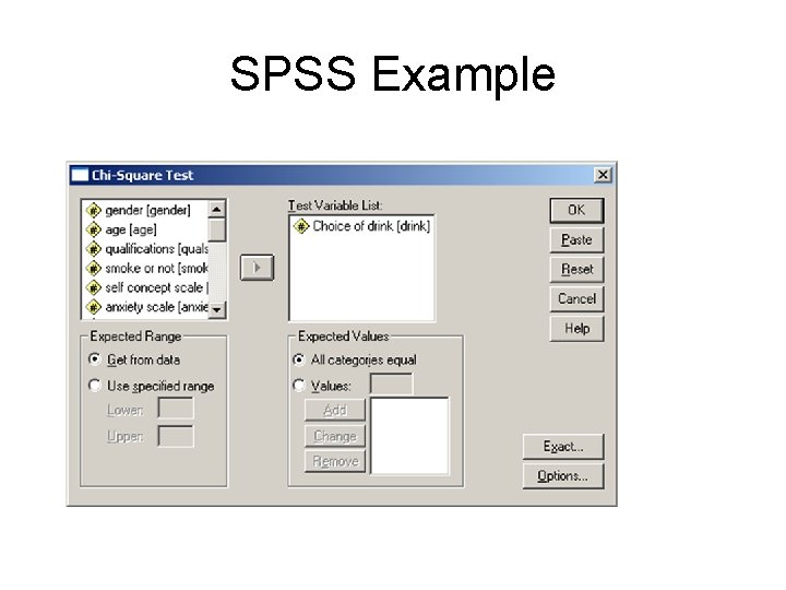
SPSS EXAMPLE OF GOODNESS OF FIT Is there any specific preference for one of three drinks? Null hypothesis claims any variation is simply random 1. Click on Analyze and select Nonparametric Tests from the drop-down menu. 2. Choose Chi-square. . . which opens the Chi. Square Test dialogue box. 3. Select the variable (in this example ‘drink’) then click on the arrow button which transfers this variable to the Test Variable List: box. 4. Select OK. The results of the analysis are displayed in next slides.

SPSS Example

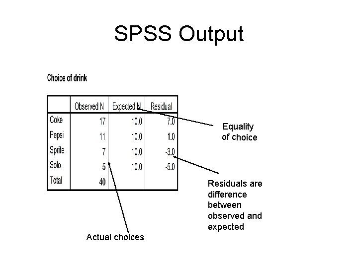
SPSS Output Equality of choice Residuals are difference between observed and expected Actual choices

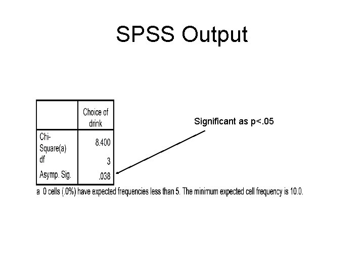
SPSS Output Significant as p<. 05

How to Interpret Output • The observed choice frequencies are presented in the second column. • The expected frequencies of cases are displayed in the third column. The expected frequency for each of the four drinks with 40 personal choices is 40/4, i. e. 10. • The residual column displays the differences between the observed and expected frequencies. • The second box presents the value of chi square, its degrees of freedom and its significance. Chi square is 8. 4, its degrees of freedom are 3 (i. e. 4 choices - 1) and its significance level is 0. 038. This indicates that there is a statistically significant deviation from the expected distribution of equality beyond p<. 05. Coke is most popular while Solo and Sprite are significantly less preferred. • Note the comment below the second sub-table. Chi square requires expected cell frequencies of at least 5.

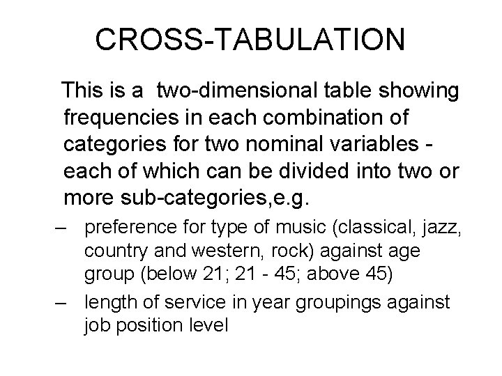
CROSS-TABULATION This is a two-dimensional table showing frequencies in each combination of categories for two nominal variables each of which can be divided into two or more sub-categories, e. g. – preference for type of music (classical, jazz, country and western, rock) against age group (below 21; 21 - 45; above 45) – length of service in year groupings against job position level

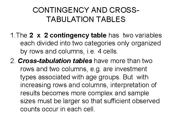
CONTINGENCY AND CROSSTABULATION TABLES 1. The 2 x 2 contingency table has two variables each divided into two categories only organized by rows and columns, i. e. 4 cells. 2. Cross-tabulation tables have more than two rows and two columns, e. g. are investment types associated with age groups. But with increasing rows and columns, interpretation of results becomes more complex and sample sizes must be larger so that sufficient observed counts occur in each cell.

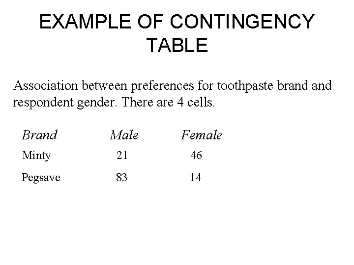
EXAMPLE OF CONTINGENCY TABLE Association between preferences for toothpaste brand respondent gender. There are 4 cells. Brand Male Female Minty 21 46 Pegsave 83 14

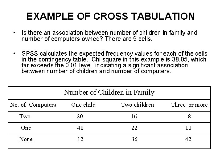
EXAMPLE OF CROSS TABULATION • Is there an association between number of children in family and number of computers owned? There are 9 cells. • SPSS calculates the expected frequency values for each of the cells in the contingency table. Chi square in this example is 38. 05, which far exceeds the 0. 01 level, indicating a significant association between number of children and number of computers. Number of Children in Family No. of Computers One child Two children Three or more Two 20 16 8 One 40 22 10 None 12 36 42

SPSS EXAMPLE OF CONTINGENCY • In this example, we will examine the Null Hypothesis that there is no significant relationship between gender and whether the person smokes or not. • The Alternate Hypothesis is that there is a significant relationship between gender and whether the person smokes or not. • The analysis compares the observed frequencies (actual data) to the expected frequencies (those that could be expected if there were no significant relationship between the two variables, i. e. frequencies possible under Ho

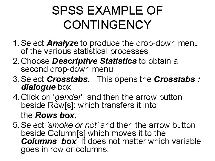
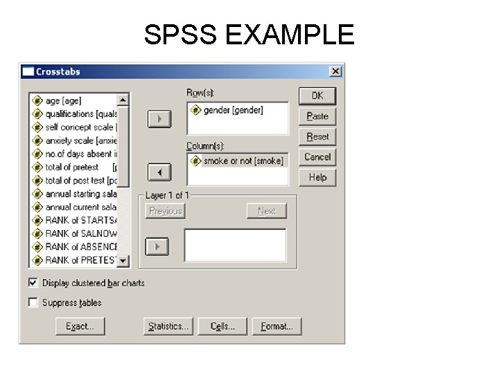
SPSS EXAMPLE OF CONTINGENCY 1. Select Analyze to produce the drop-down menu of the various statistical processes. 2. Choose Descriptive Statistics to obtain a second drop-down menu 3. Select Crosstabs. This opens the Crosstabs : dialogue box. 4. Click on ‘gender' and then the arrow button beside Row[s]: which transfers it into the Rows box. 5. Select 'smoke or not' and then the arrow button beside Column[s] which moves it to the Columns box. It does not matter which variable goes in row or columns.

SPSS EXAMPLE

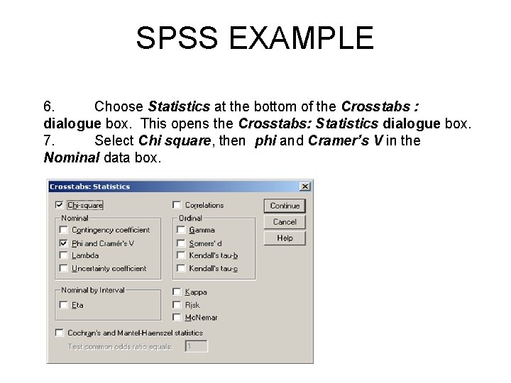
SPSS EXAMPLE 6. Choose Statistics at the bottom of the Crosstabs : dialogue box. This opens the Crosstabs: Statistics dialogue box. 7. Select Chi square, then phi and Cramer’s V in the Nominal data box.

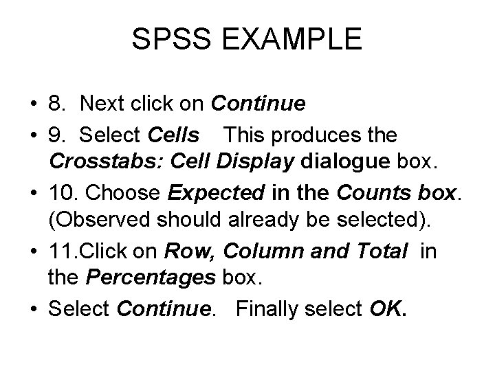
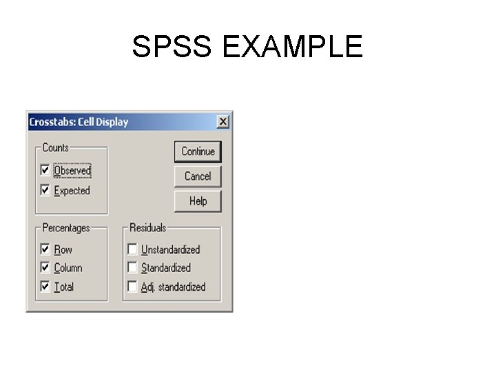
SPSS EXAMPLE • 8. Next click on Continue • 9. Select Cells This produces the Crosstabs: Cell Display dialogue box. • 10. Choose Expected in the Counts box. (Observed should already be selected). • 11. Click on Row, Column and Total in the Percentages box. • Select Continue. Finally select OK.

SPSS EXAMPLE

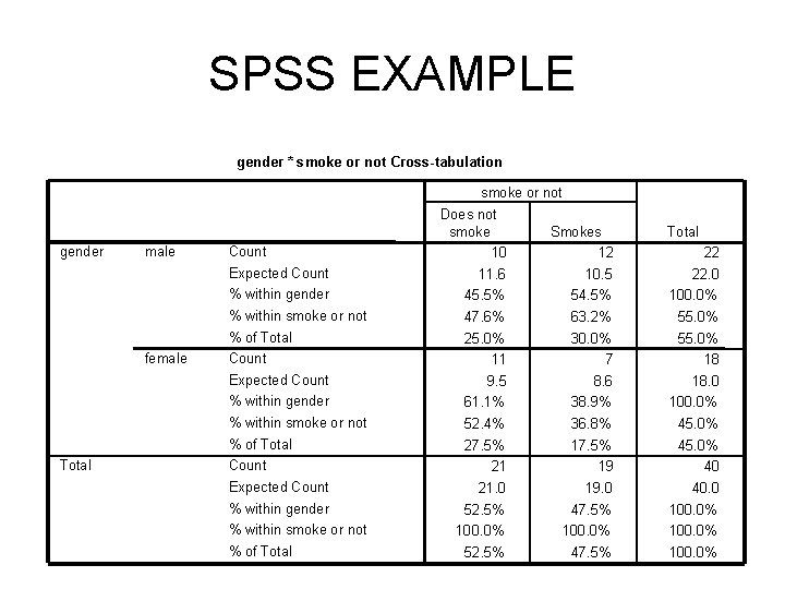
SPSS EXAMPLE gender * smoke or not Cross-tabulation smoke or not gender male female Total Does not smoke 10 Smokes 12 Expected Count 11. 6 10. 5 22. 0 % within gender 45. 5% 54. 5% 100. 0% % within smoke or not 47. 6% 63. 2% 55. 0% % of Total 25. 0% 30. 0% 55. 0% 11 7 18 Expected Count 9. 5 8. 6 18. 0 % within gender 61. 1% 38. 9% 100. 0% % within smoke or not 52. 4% 36. 8% 45. 0% % of Total 27. 5% 17. 5% 45. 0% 21 19 40 Expected Count 21. 0 19. 0 40. 0 % within gender 52. 5% 47. 5% 100. 0% 52. 5% 47. 5% 100. 0% Count % within smoke or not % of Total 22

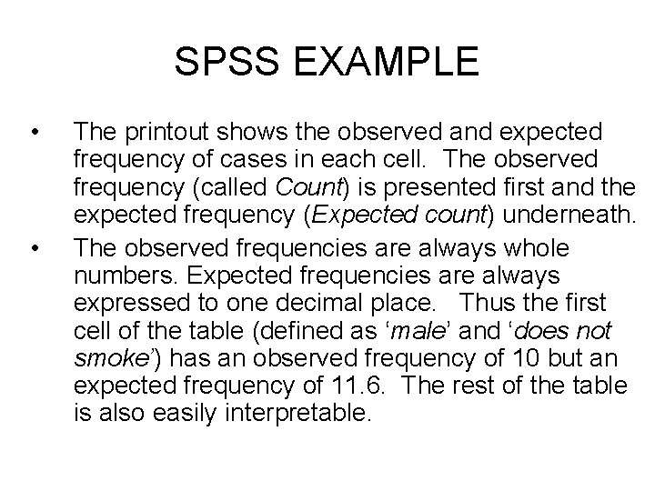
SPSS EXAMPLE • • The printout shows the observed and expected frequency of cases in each cell. The observed frequency (called Count) is presented first and the expected frequency (Expected count) underneath. The observed frequencies are always whole numbers. Expected frequencies are always expressed to one decimal place. Thus the first cell of the table (defined as ‘male’ and ‘does not smoke’) has an observed frequency of 10 but an expected frequency of 11. 6. The rest of the table is also easily interpretable.

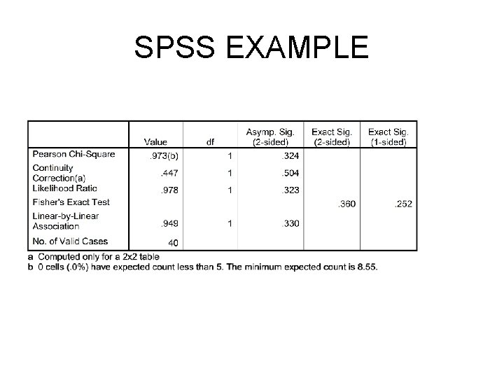
SPSS EXAMPLE

SPSS EXAMPLE • This table displays the chi-square value, its degrees of freedom and significance level. Chi square is on the line labelled ‘Pearson’ with a value of 0. 973. Its degrees of freedom are 1 and its two-tailed probability is 0. 324. There is no significant association between smoking and gender. Ho is retained. • Note the warning about the Minimum Expected Frequency of any cell in the table. If there are cells with a minimum expected frequency of 5. 0 or less then we should be wary of using chi square and use Fisher’s Exact test result instead which will be produced by SPSS in such cases.

SPSS EXAMPLE • If a significant result is obtained, you must refer back to the Cross-tabulation table in order to interpret what the significant pattern is and means • Look at the patterns between observed and expected, for they provide the information of what associations exist and their direction

RESTRICTIONS IN THE USE OF THE CHI SQUARE • chi square is only appropriate for data that are classified as frequency of occurrence (counts) within categories (nominal data) • it must only be used on frequencies, never on percentages • categories must be mutually exclusive - each response can be classified into only one cell • larger samples are needed when there are many categories within each variable. – A rule-of-thumb is that the expected frequency in all cells should at least equal or be greater than 5. – Fusing of categories is not really desirable, since it involves a reduction in the amount of information available.

SUMMARY OF STEPS IN CHI SQUARE • Null and alternate hypotheses about the proposed relationship are stated • We compute frequencies of occurrence of events that we expect under the null hypothesis to provide the expected frequencies for each cell • We note the computed chi square in the SPSS printout and whether statistical significance is achieved • We inspect our original data to determine the direction of association if a significant result is obtained