Chemical Bonding II Molecular Shapes Valence Bond Theory

Chemical Bonding II Molecular Shapes, Valence Bond Theory, and Molecular Orbital Theory

Goals in this Unit • Learn the basic shapes in chemical bonding. • See how these lead to molecular geometries. • Understand the predictive powers of the model. • Molecular shape as it relates to polarity. • The valence bond model and the MO model— different ways to solve the same equation!

VSEPR Theory. . . Valence Shell Electron Pair Repulsion

Basic Idea Repulsion between electrons (pairs, usually) determine molecular geometry.

Basic Shapes Arising from Model Two dimensional: Linear Trigonal Planar Three dimensional: Tetrahedral Trigonal bipyrmidal Octahedral

Think about this as “objects” abount an atom. What are “objects”? Electron pairs Bonds Single, double, and triple objects count as just single objects! As we go along, we shall look especially at bond angles!

Two Electron Groups: Linear Geometry

Three Electron Groups: Trigonal Planar Geometry As Lewis Structure Actual Geometry

NO 3 -: another good example (Note: Resonance Form)

On-board Example Ozone

Four Electron Groups: Tetrahedral Geometry (Introduction)

Thing to note in next slide. . . • Lewis structure is 2 D. • Actual molecular structure must be 3 D!

Classic Prototype: Methane

Before going on. . . • Electron geometry and • Molecular shape • should not be confused! • Consider ammonia. . .

Consider these carefully!

For that matter. . .

Five Electron Groups

PCl 5: A typical example

Six Electron Groups

SF 6: An excellent example!

A Deeper Discussion of Lone Pairs • Presence of lone pairs makes us think a little bit more. • We now really look at the difference between electronic geometry and molecular geometry! • General rule: Lone pairs repel each other more strongly than bonded pairs. • Why would this be?

Here is a partial explanation. . .

This causes changes in bond angles. . . • We look at progressive changes using tetrahedral electronic structures as an example. • We do these on the board. . . • CH 4 • NH 3 • H 2 0

5 electron groups even more p. Hun! • Let us first look at SF 4. • Here we have 5 electron groups with just one lone pair. • Two structures can be imagined but only one occurs. . . • p. Hirst, we draw the Lewis structure on the board. . . • And, then, . . .

With 5 -electron groups, we can have T shapes. . .

And, even a linear shape!

On to the joys of 6 -coordinate geometry! • We shall look at a few examples here. • We shall explain each slide verbally as we go.

As single lone pair as in. . .

. . . leads to. . .

Two lone pairs are even more fun!

A Summary of VSEPR Model • Geometry of a molecule determined by the number electron groups on central and interior atoms. • The number of electrons can be determined by the Lewis structure. • Each of the following is considered to be an electron group: lone pair, single bond, double bond, triple bond.

Summary, continued. . . • Molecular geometry determined by repulsion strengths. • In general, Lone pair—lone pair > lone pair— bonding pair > bonding pair—bonding pair • Bond angles vary from idealized angles because double and triple bonds are larger than single bonds and lone pairs are even larger.

Reconciling 2 D and 3 D. . .

Putting this into practice. . .

This all really gets to be p. Hun when we get into organic structures. . .

Translation of Lewis 2 D to molecular 3 D. . .

Molecular Shape & Polarity The return of electronegatvities!

On obvious case: A heteronuclear diatomic molecule. . .

Bond dipole moments. . . • If ∆�� ≠ 0 between to atoms, then we can have a bond dipole moment. • Bond dipole moments are vectors and add according to the rules of vector algebra. • Dipole moments and cancel each other out or reinforce each other. • We give some examples now. . .

μ-vectors cancel in CO 2

μ-vectors add to give a net μ in H 2 O

A little cursory discussion. . .

VB & MO Methods • Both methods are solving Hψ = Eψ. • They go about it in different ways. • Valence bond (VB) stresses localized AO’s before combining to get ψ. • Molecular orbital theory uses delocalized MO’s (LCAO) to set up ψ. • These are vague descriptions here but we shall try to make them clearer as we go!

Simple Example: Formation of H 2

Some Details about VB Theory • Electrons reside in quantum-mechanical orbitals localized on individual atoms. • The orbitals are overlapping atomic orbitals from adjoining (bonded) atoms. • These can be the usual s, p, and d AO’s from the individual atoms • OR • they can be hybridized atomic orbitals. • The overlapping is what leads to a chemical bond.

H 2 S: An example of simple AO overlap Individual AO’s Overlapping to make bonds

How Lewis & VB Theory Differ Lewis Theory Here, a chemical bond is simply a pair of shared electrons. We represent these as a pair of dots (or a single dash). VB Theory A chemical bond is formed by the overlap of two half-filled atomic orbitals. The bond is sometimes referred to as a localized molecular orbital. Note that this is sometimes misleading!

Why we need to hybridize AO’s Consider C & H AO’s Naive view leads to. . .

But. . . The reality is this-- Yes! The theory must fit the facts!

Hybrid Orbitals • Atomic orbitals with the same principal quantum number (n) can be combined to make what we call hybrid orbitals. • Orbitals that can be combined are called degenerate orbitals. • The hybrid orbitals are also degenerate. • But. . .

Some rules for hybridization • The number of standard AO’s added together always gives the same number of hybrid AO’s. • The particular combinations of standard AO’s determine the shapes and energies of the hybrids. • The particular hybridization that occurs is that which yields the lowest overall energy for the molecule (or molecular fragment).

Hybrid types & molecular geometry We list the types now and their corresponding geometries before going on into details. . . sp 3 sp 2 sp sp 3 d 2 Tetrahedral Trigonal planar Linear Trigonal bipyramid Octahedral

sp 3 Hybridization

Examples of this in action! Methane Ammonia

sp 2 Hybridization

The formation is like this. . .

What about the extra p orbital?

The extra p orbitals on each atom • overlap to make a second bond! • The bond from the overlapping hybrids is called a σ bond (sigma bond) • and • the second bond has the unhybridized p orbitals overlap to give a • π bond! (pi bond)

An example: Formaldehyde

Geometrical Significance of Single- vs. Double-Bonds 1, 2 -Dichloroethane cis-1, 2 -Dichloroethene

Double bonding can lead to isomers!

A photochemical aside • A photon can impinge upon a double bond and temporarily break the π bond. • This allows for isomerization. • The next example, from the book, shows the isomerization of 11 -cis-retinal and all-transretinal that occurs in your eyes. • The isomerization triggers an electrical impulse to your brain.

Here are the two forms of retinal!

sp Hybridization occurs from this. . .

Or, you can look at it this way. . .

The unhybridized p orbitals get to participate in making triple bonds!

Here is how sp 3 d hybrids form. . .

We show the “orbital manifold”. . .

Here is an example along with its Lewis structure. . .

sp 3 d 2 is quite similar. . .

Here is the orbital manifold. . .

And, here is an example complete with a Lewis structure companion. . .

What do you suppose this is? (Hint: Mo 2 is the molecule!)

Summary of Geometries & Hybridization Schemes

Molecular Orbital Theory VB Theory: Hybrid orbitals are weighted linear sums of atomic orbitals on a given atom. We are working with localized entities. MO Theory: MO’s are weighted linear sums of atomic orbitals from all the atoms. We are working with delocalized entities.

General Comments • Orbitals combine so that the energy of the entire molecule is made to be as low as possible. • Computations involve using trial wave functions to get as good an approximate solution to the Schrödinger equation as possible by minimizing the energy. • This is called the variation method.

How MO’s are made. . . • We use LCAO (Linear Combination of Atomic Orbitals) to make MO’s. • The MO’s, in turn, are combined to give the entire molecular wave function, ψ. • The sets of coefficients in each MO are adjusted by the variation method to give the best (lowest) energy. • This, then, gives a numerical solution to the Schrödinger equation.

A Simple Example: H 2 • The 1 s AO’s of each H combine to give two MO’s. . . – One is a bonding orbital. – The other is an antibonding orbital. • This ties in to the wave nature of electron motion. – Bonding orbitals → Constructive Interference – Antibonding orbitals → Destructive interference

This is what we are talking about!

Here is another way to express it!

Note the language and notation. . .

We can envision this via an energy level diagram. . .

Some points. . . • With H 2, we have two electrons and two MO’s. • The MO’s fill in just the same way as we saw earlier with AO’s in atoms. • Electrons are paired (only two allowed to a molecular orbital). • So, we now have (sort of) a molecular Aufbau Principle! • The usual ordering and Hund’s rule are obeyed.

The concept of the bond is altered! • Bonds are now defined via how many electrons are in bonding and antibonding MO’s. • We get what is called Bond Order. • It is given by a simple formula:

For example. . . For H 2, the bond order is just In other words, we have a single bond!

Carrying this idea further, we see why He 2 doe not exist!

Surprise! He 2+ is predicted to exist! And, it does! (But not happily!)

This exists, too, and is isoelectronic to the previous example. . .

We have been looking at heteronuclear diatomic molecules • Let’s look at the next two in the periodic table, namely, Li 2 and Be 2. • We note that 2 s atomic orbitals combine to give σ2 s and σ2 s*. • These fill as the examples we just saw. . .

Li 2

One guy is skeptical about this being dilithium. . .

Diberyllium is not stable—and this is no surprise!

Now, let’s continue! But. . . We have run out of s orbitals? What do we do? Well, between two atoms, we have 6 p orbitals. • These combine to give 6 π orbitals! • And, these, in turn come in two flavors! • •

End-on alignment gives these

Another view: With phase

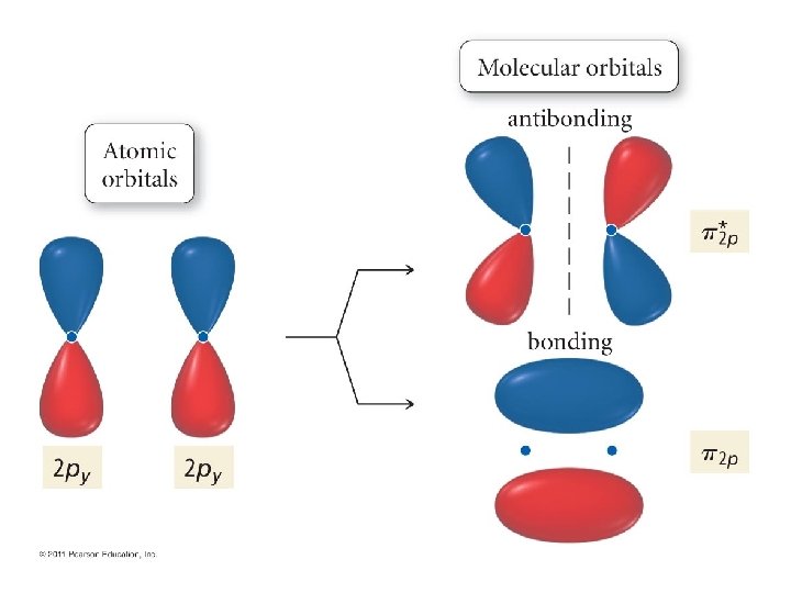
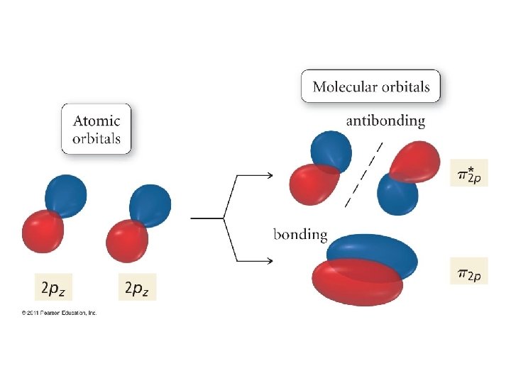
Parallel alignment gives these. . .

. . . and these!

We look at these now, with phase included. . .

So, we now have 6 more MO’s we can fill!

We briefly discuss the energy ordering. . . • Mixing of orbitals changes as we add more electrons. • That is, 2 s-2 p interactions affect the MO energies. • Needless to say, this is difficult to understand at an elementary level!

Let’s now look at the rest of our happy family of diatomic molecules!

The strange and curious case of oxygen, O 2 • Oxygen is paramagnetic! • This is not clear from the Lewis and VB models. • But, it follows quite easily from the MO model since two degenerate antibonding MO’s can have only one electron each. • And these electrons have to be parallel in spin. • In other words, Hund’s rule comes to the fore!

Let’s compare the models. . .

This is confirmed by experiment. . .

Heteronuclear Molecules • Most molecules we know consist of more than one type of element. • The term we use with such is heteronuclear. • These form in much the same way, but the atomic orbitals start out with different energies. • We see this in the next slide.

Two simple examples. . .

Major point. . . • More electronegative atoms have lower electronic energies. • Thus, electrons gravitate toward them. • This is a natural explanation of bond polarity!

MO Theory vs. Resonance • Resonance does not appear in MO theory. • This is because the electrons are already delocalized! • VB can get the same thing—but only by superimposing structures. • We look at some examples now. . .