Characterization of Forecast Error using Singular Value Decomposition

Characterization of Forecast Error using Singular Value Decomposition Andy Moore and Kevin Smith University of California Santa Cruz Hernan Arango Rutgers University

Outline • An overview of singular value decomposition (SVD) • Flavors of SVD • Duality of SVD • Norms • Unstable jet • California Current

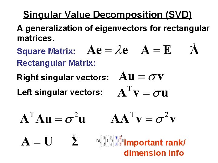
Singular Value Decomposition (SVD) A generalization of eigenvectors for rectangular matrices. Square Matrix: Rectangular Matrix: Right singular vectors: Left singular vectors: Important rank/ dimension info

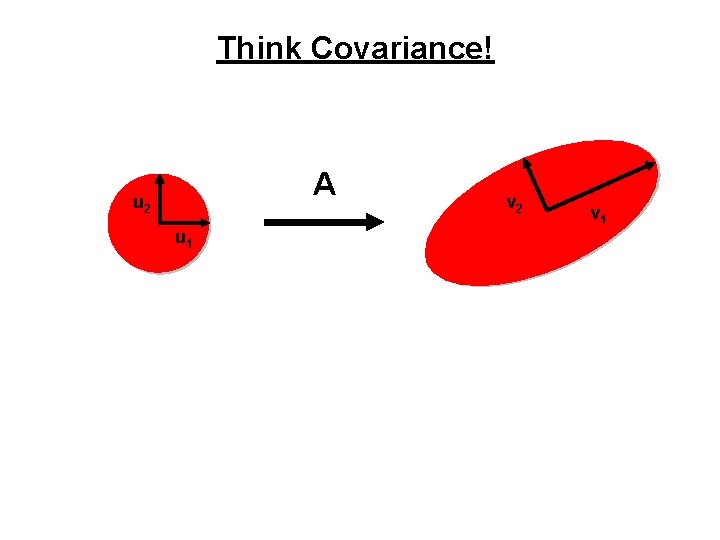
Think Covariance! A u 2 u 1 v 2 v 1

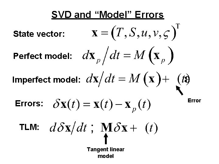
SVD and “Model” Errors State vector: Perfect model: Imperfect model: Errors: TLM: Tangent linear model

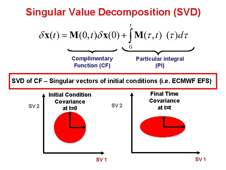
Singular Value Decomposition (SVD) Complimentary Function (CF) Particular integral (PI) SVD of CF – Singular vectors of initial conditions (i. e. ECMWF EFS) SV 2 Initial Condition Covariance at t=0 SV 2 SV 1 Final Time Covariance at t=t SV 1

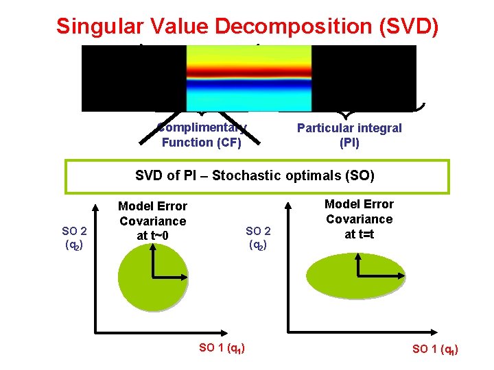
Singular Value Decomposition (SVD) Complimentary Function (CF) Particular integral (PI) SVD of PI – Stochastic optimals (SO) SO 2 (q 2) Model Error Covariance at t~0 SO 2 (q 2) SO 1 (q 1) Model Error Covariance at t=t SO 1 (q 1)

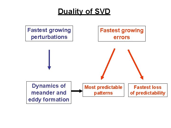
Duality of SVD Fastest growing perturbations Dynamics of meander and eddy formation Fastest growing errors Most predictable patterns Fastest loss of predictability

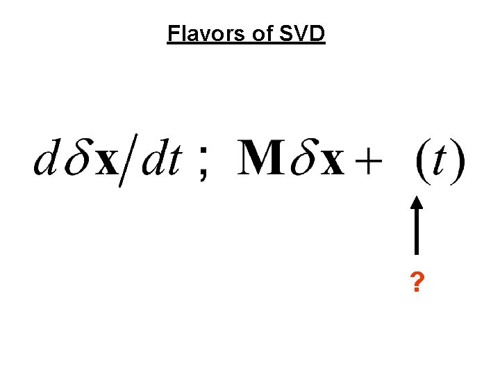
Flavors of SVD ?

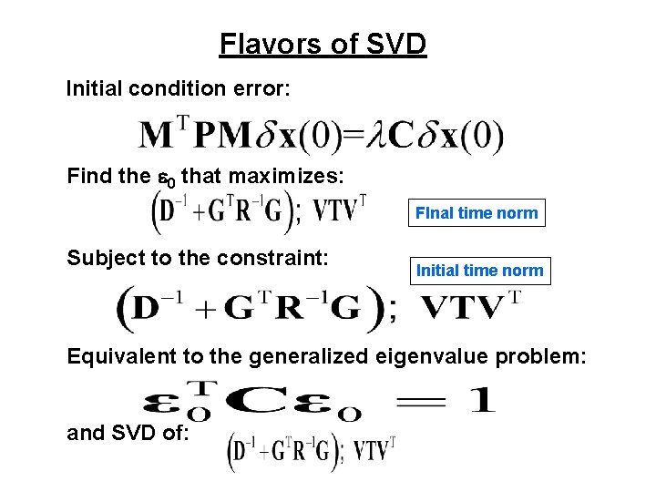
Flavors of SVD Initial condition error: Find the e 0 that maximizes: FInal time norm Subject to the constraint: Initial time norm Equivalent to the generalized eigenvalue problem: and SVD of:

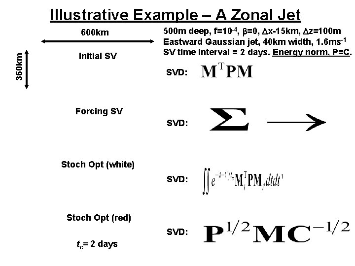
Illustrative Example – A Zonal Jet 360 km 600 km Initial SV 500 m deep, f=10 -4, b=0, Dx-15 km, Dz=100 m Eastward Gaussian jet, 40 km width, 1. 6 ms-1 SV time interval = 2 days. Energy norm, P=C. SVD: Forcing SV SVD: Stoch Opt (white) SVD: Stoch Opt (red) SVD: tc= 2 days

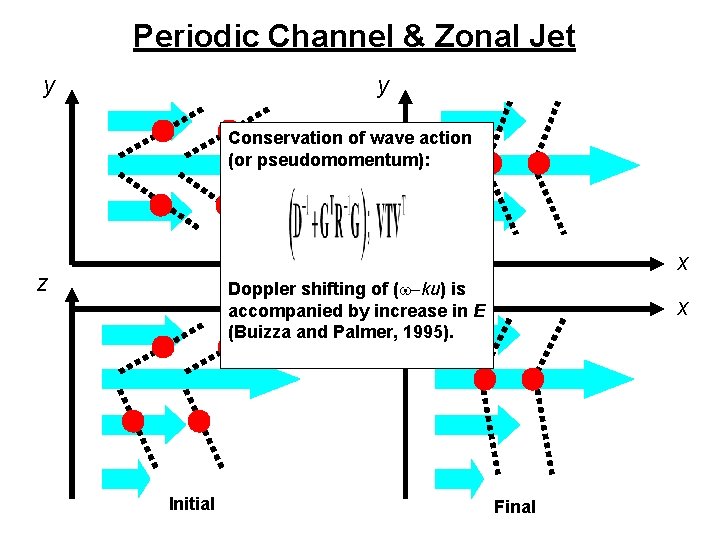
Periodic Channel & Zonal Jet y y Conservation of wave action (or pseudomomentum): x z x Doppler shifting z of (w-ku) is accompaniedxby increase in E (Buizza and Palmer, 1995). Initial x Final

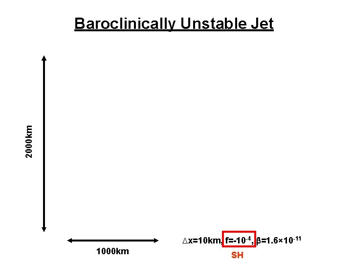
Baroclinically Unstable Jet t=50 days SST 2000 km t=0 Dx=10 km, f=-10 -4, b=1. 6× 10 -11 1000 km SH

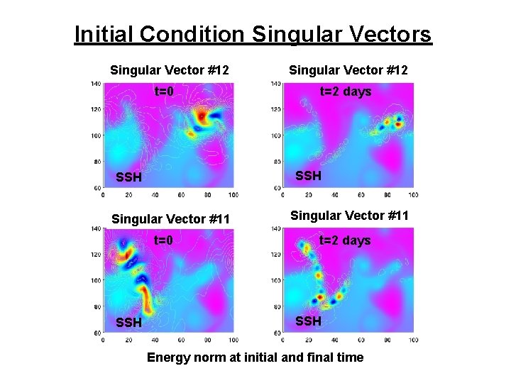
Initial Condition Singular Vectors Singular Vector #12 t=0 t=2 days SSH Singular Vector #11 t=0 SSH Singular Vector #12 Singular Vector #11 t=2 days SSH Energy norm at initial and final time

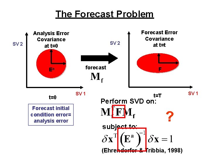
The Forecast Problem SV 2 Analysis Error Covariance at t=0 Ea t=0 Forecast initial condition error= analysis error SV 2 Forecast Error Covariance at t=t forecast SV 1 F SV 1 t=T Perform SVD on: subject to: ? (Ehrendorfer & Tribbia, 1998)

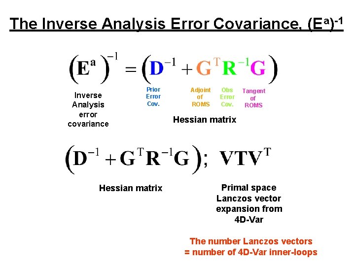
The Inverse Analysis Error Covariance, (Ea)-1 Inverse Analysis error covariance Prior Error Cov. Hessian matrix Adjoint of ROMS Obs Error Cov. Tangent of ROMS Hessian matrix Primal space Lanczos vector expansion from 4 D-Var The number Lanczos vectors = number of 4 D-Var inner-loops

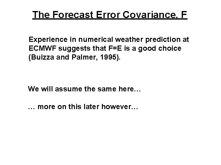
The Forecast Error Covariance, F Experience in numerical weather prediction at ECMWF suggests that F=E is a good choice (Buizza and Palmer, 1995). We will assume the same here… … more on this later however…

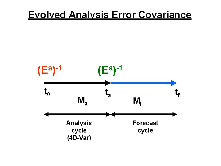
Evolved Analysis Error Covariance (Ea)-1 t 0 (Ea)-1 Ma Analysis cycle (4 D-Var) ta Mf Forecast cycle tf

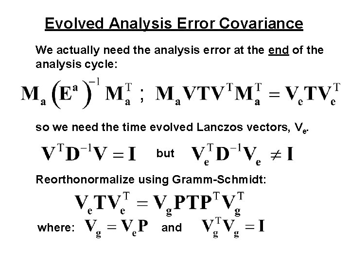
Evolved Analysis Error Covariance We actually need the analysis error at the end of the analysis cycle: so we need the time evolved Lanczos vectors, Ve. but Reorthonormalize using Gramm-Schmidt: where: and

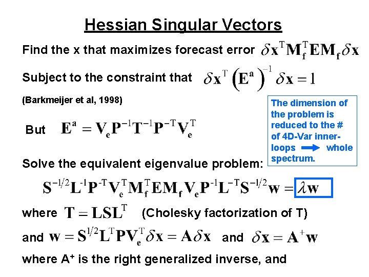
Hessian Singular Vectors Find the x that maximizes forecast error Subject to the constraint that (Barkmeijer et al, 1998) But Solve the equivalent eigenvalue problem: where and The dimension of the problem is reduced to the # of 4 D-Var innerloops whole spectrum. (Cholesky factorization of T) and where A+ is the right generalized inverse, and

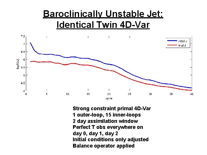
Baroclinically Unstable Jet: Identical Twin 4 D-Var Strong constraint primal 4 D-Var 1 outer-loop, 15 inner-loops 2 day assimilation window Perfect T obs everywhere on day 0, day 1, day 2 Initial conditions only adjusted Balance operator applied

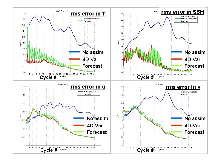
rms error in SSH rms error in T No assim 4 D-Var Forecast Cycle # rms error in u rms error in v No assim 4 D-Var Forecast Cycle #

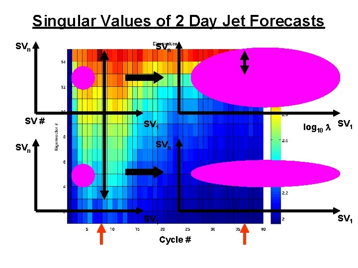
Singular Values of 2 Day Jet Forecasts SVn SV # SVn SV 1 log 10 l SV 1 SVn SV 1 Cycle # SV 1

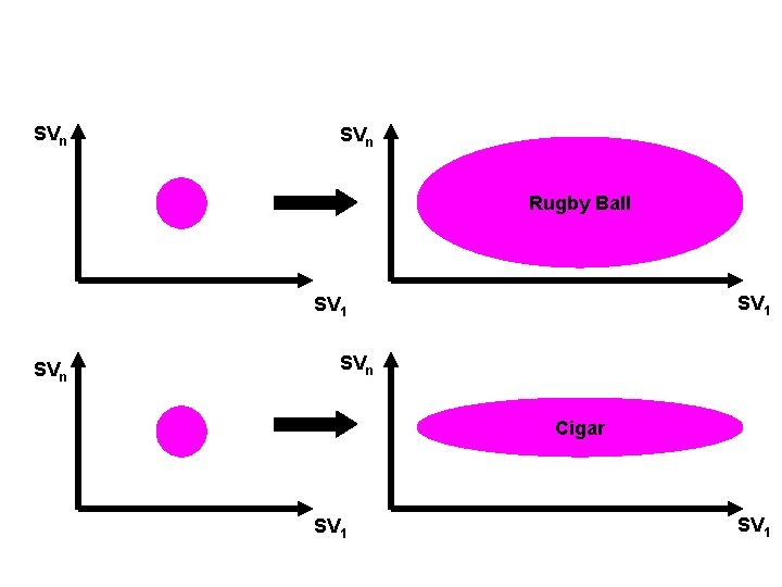
SVn Rugby Ball SV 1 SVn Cigar SV 1

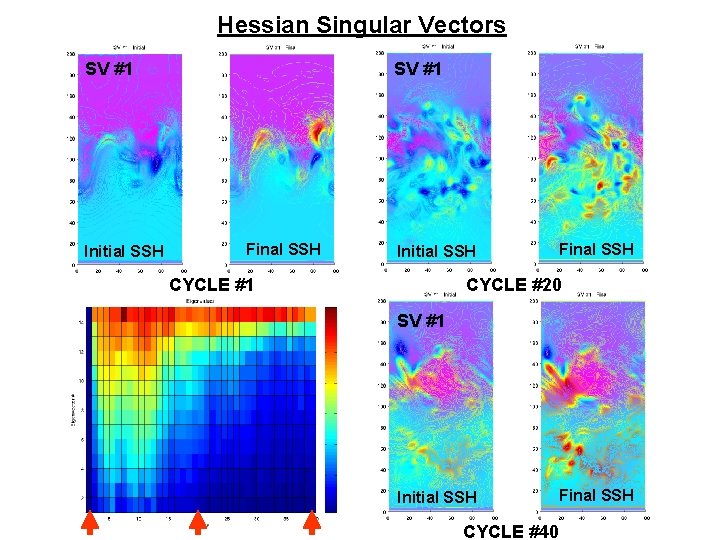
Hessian Singular Vectors SV #1 Initial SSH SV #1 Final SSH Initial SSH CYCLE #1 Final SSH CYCLE #20 SV #1 Initial SSH Final SSH CYCLE #40

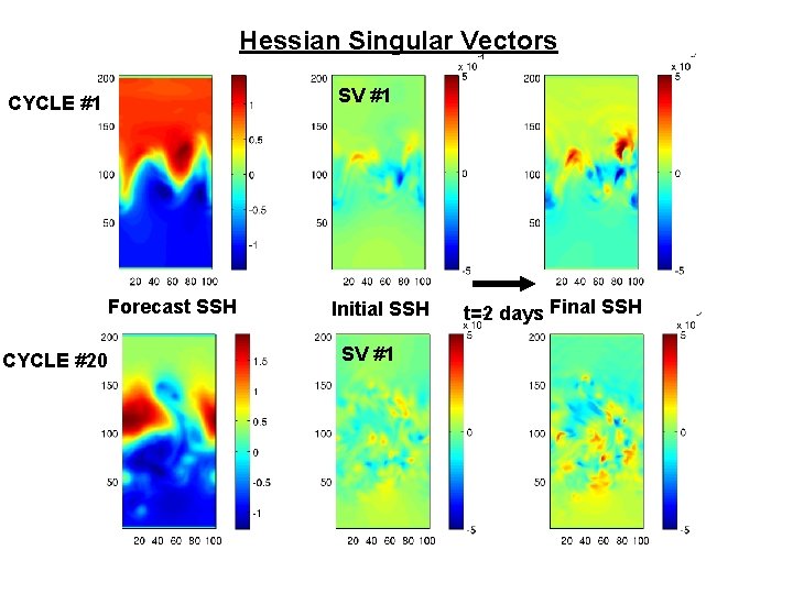
Hessian Singular Vectors SV #1 CYCLE #1 Forecast SSH CYCLE #20 Initial SSH SV #1 t=2 days Final SSH

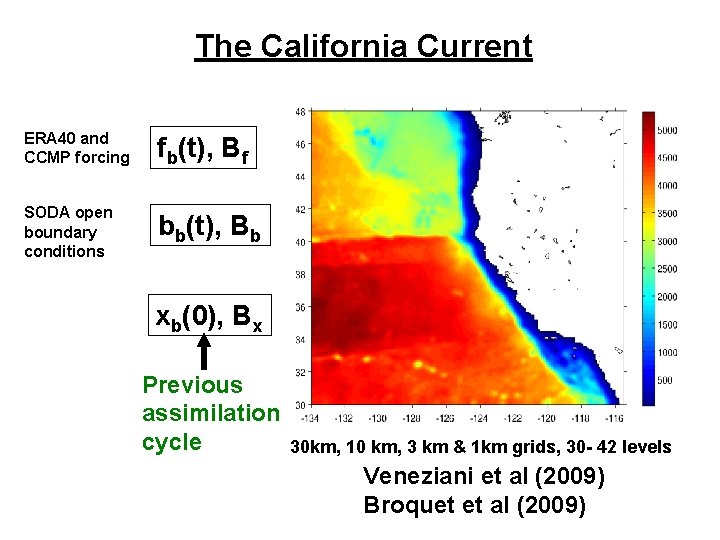
The California Current ERA 40 and CCMP forcing fb(t), Bf SODA open boundary conditions bb(t), Bb xb(0), Bx Previous assimilation cycle 30 km, 10 km, 3 km & 1 km grids, 30 - 42 levels Veneziani et al (2009) Broquet et al (2009)

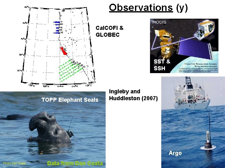
Observations (y) Cal. COFI & GLOBEC SST & SSH TOPP Elephant Seals Ingleby and Huddleston (2007) Argo Data from Dan Costa

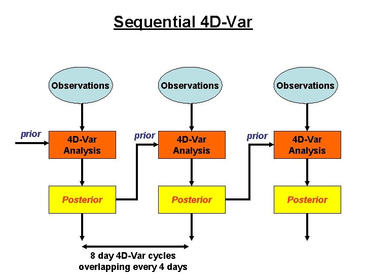
Sequential 4 D-Var Observations prior 4 D-Var Analysis Posterior 8 day 4 D-Var cycles overlapping every 4 days Observations prior 4 D-Var Analysis Posterior

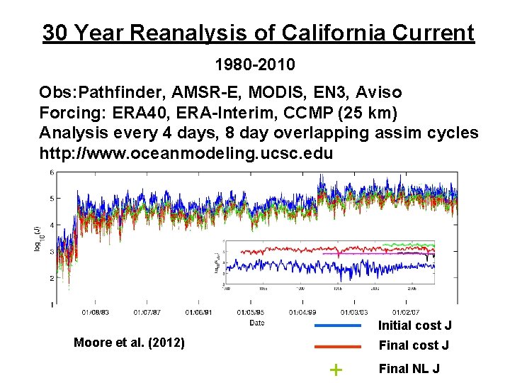
30 Year Reanalysis of California Current 1980 -2010 Obs: Pathfinder, AMSR-E, MODIS, EN 3, Aviso Forcing: ERA 40, ERA-Interim, CCMP (25 km) Analysis every 4 days, 8 day overlapping assim cycles http: //www. oceanmodeling. ucsc. edu Initial cost J Moore et al. (2012) Final cost J + Final NL J

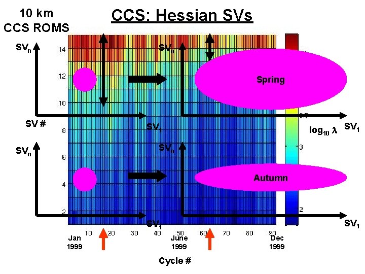
10 km CCS ROMS SVn CCS: Hessian SVs SVn Spring SV # log 10 l SV 1 SVn Autumn SV 1 Jan 1999 June 1999 Cycle # Dec 1999

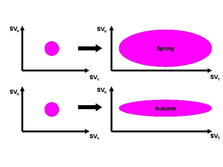
SVn Spring SV 1 SVn Autumn SV 1

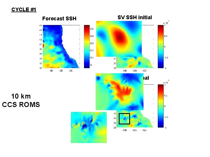
CYCLE #1 Forecast SSH SV SSH initial SV SSH final 10 km CCS ROMS

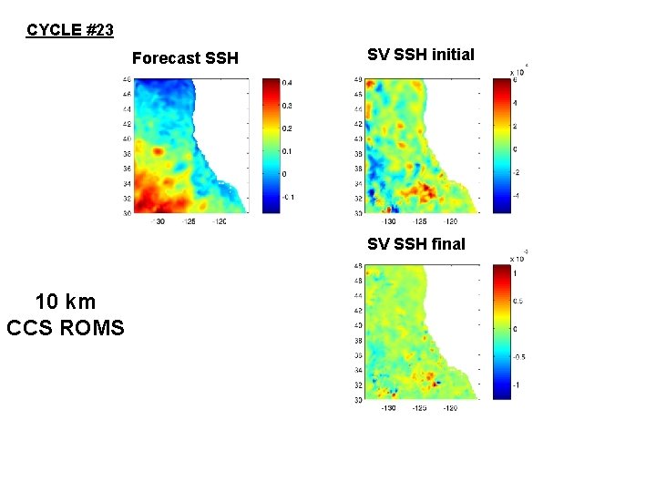
CYCLE #23 Forecast SSH SV SSH initial SV SSH final 10 km CCS ROMS

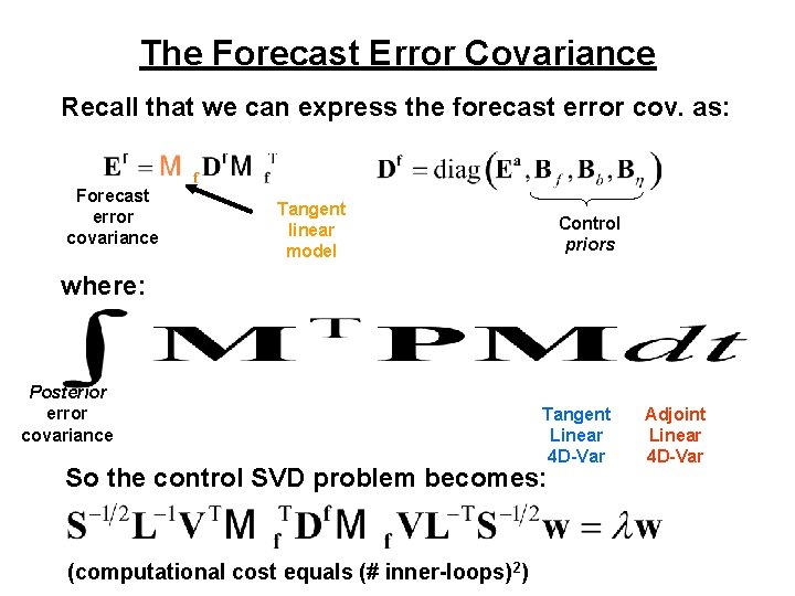
The Forecast Error Covariance Recall that we can express the forecast error cov. as: Forecast error covariance Tangent linear model Control priors where: Posterior error covariance Tangent Linear 4 D-Var So the control SVD problem becomes: (computational cost equals (# inner-loops)2) Adjoint Linear 4 D-Var

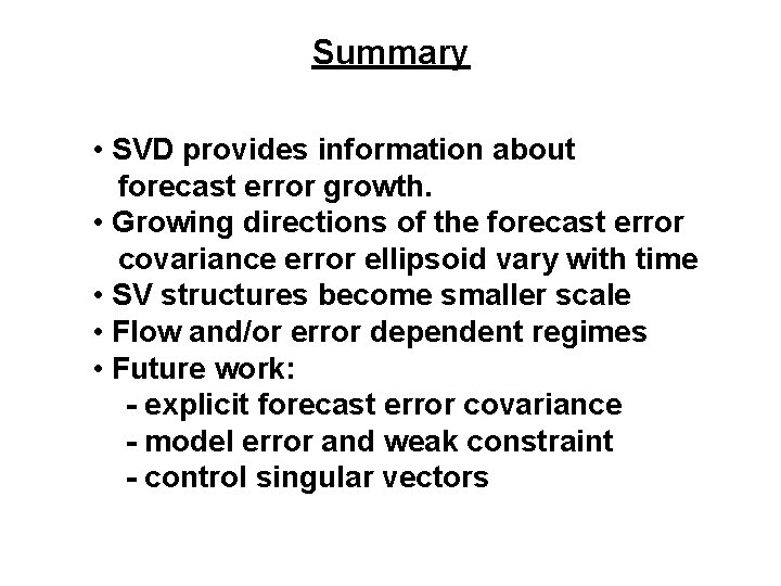
Summary • SVD provides information about forecast error growth. • Growing directions of the forecast error covariance error ellipsoid vary with time • SV structures become smaller scale • Flow and/or error dependent regimes • Future work: - explicit forecast error covariance - model error and weak constraint - control singular vectors